Download
1 / 54
540 likes | 661 Views
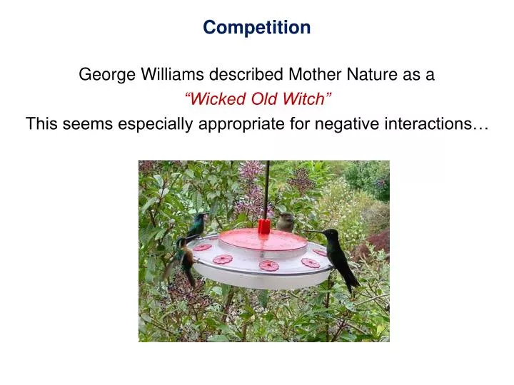
George Williams described Mother Nature as a “Wicked Old Witch” This seems especially appropriate for negative interactions…. Competition. Competition.

E N D
George Williams described Mother Nature as a “Wicked Old Witch” This seems especially appropriate for negative interactions… Competition
Competition Competition (generally an intra-trophic level phenomenon) occurs when each species negatively influences the population growth rate (or size) of the other This phenomenological definition is used in the modeling framework proposed by AlfredLotka (1880-1949) & VitoVolterra (1860-1940) Their shared goal was to determine the conditions under which competitive exclusion vs. coexistence would occur between two sympatric competitors
Population Dynamics ∆N Exponential growth = r • N ∆t Occurs when growth rate is proportional to population size; Requires unlimited resources N Time
Population Dynamics & death (d) rates Density-dependent per capita birth (b) Notice that per capita fitness increases with decreases in population size from K b b r or d d Equilibrium (= carrying capacity, K) N
Population Dynamics ∆N N Logistic growth = r • N • (1 – ) ∆t K K = carrying capacity = 0 N is maximized ∆N ∆N ∆N = 0 ∆t ∆t ∆t Time
Competition Lotka-Volterra Competition Equations: In the logistic population growth model, the growth rate is reduced by intraspecific competition: Species 1: dN1/dt = r1N1[(K1-N1)/K1] Species 2: dN2/dt = r2N2[(K2-N2)/K2] Lotka & Volterra’s equations include functions to further reduce growth rates as a consequence of interspecific competition: Species 1: dN1/dt = r1N1[(K1-N1-f(N2))/K1] Species 2: dN2/dt = r2N2[(K2-N2-f(N1))/K2]
Competition Lotka-Volterra Competition Equations: The function (f) could take on many forms, e.g.: Species 1: dN1/dt = r1N1[(K1-N1-αN2)/K1] Species 2: dN2/dt = r2N2[(K2-N2-βN1)/K2] The competition coefficientsα & β measure the per capita effect of one species on the population growth of the other, measured relative to the effect of intraspecific competition If α = 1, then per capita intraspecific effects = interspecific effects If α < 1, then intraspecific effects are more deleterious to Species 1 than interspecific effects If α > 1, then interspecific effects are more deleterious
2 2 1 2 1 2 1 1 1 1 1 1 1 Area within the frame represents carrying capacity (K) of either species The size of each square is proportional to the resources an individual consumes and makes unavailable to others (Sp. 1 = purple, Sp. 2 = green) Individuals of Sp. 2 consume 4x resources consumed by individuals of Sp. 1 For Species 1: dN1/dt = r1N1[(K1-N1-αN2)/K1] … where α = 4. Redrawn from Gotelli (2001)
2 2 1 2 1 2 1 1 1 1 1 1 1 Competition is occurring because both α & β > 0 α = 4 & β = ¼ In this case, adding an individual of Species 2 is more deleterious to Species 1 than is adding an individual of Species 1… but, adding an individual of Species 1 is less deleterious to Species 2 than is adding an individual of Species 2 Redrawn from Gotelli (2001)
2 2 1 2 1 2 1 1 1 1 1 1 1 Asymmetric competition In this case: α > β α> 1 β < 1
1 2 2 1 2 2 1 Asymmetric competition In this case: α > β α> 1 β = 1 Asymmetric competition can occur throughout the spectrum of: αβ, (α < = > 1, or β < = > 1) What circumstances might the figure above represent? Exclusively interspecific territoriality, intra-guild predation…
1 2 2 1 2 2 1 Symmetric competition In this case: α = β = 1, i.e., the special case of competitive equivalence Symmetric competition can occur throughout the spectrum of: (α=β) < = > 1
However, each species’ equilibrium depends on the equilibrium of the other species! So, by substitution… Species 1: N1 = K1 - α(K2 - βN1) Species 2: N2 = K2 - β(K1 - αN2) ^ ^ ^ ^ Lotka-Volterra Phenomenological Competition Model Find equilibrium solutions to the equations, i.e., set dN/dt = 0: Species 1: N1 = K1 - αN2 Species 2: N2 = K2 - βN1 ^ ^ This makes intuitive sense: The equilibrium for N1 is the carrying capacity for Species 1 (K1) reduced by some amount owing to the presence of Species 2 (αN2)
Lotka-Volterra Phenomenological Competition Model The equations for equilibrium solutions become: Species 1: N1 = [K1 - αK2] / [1 - α β] Species 2: N2 = [K2 - βK1] / [1 - α β] ^ ^ These provide some insights into the conditions required for coexistence under the assumptions of the model E.g., the product αβ must be < 1 for N to be > 0 for both species (a necessary condition for coexistence) But they do not provide much insight into the dynamics of competitive interactions, e.g., are the equilibrium points stable?
4 time steps State-space graphs help to track population trajectories (and assess stability) predicted by models Mapping state-space trajectories onto single population trajectories From Gotelli (2001)
4 time steps State-space graphs help to track population trajectories (and assess stability) predicted by models 4 time steps Mapping state-space trajectories onto single population trajectories From Gotelli (2001)
Lotka-Volterra Model Remember that equilibrium solutions require dN/dt = 0 Species 1: N1 = K1 - αN2 ^ Therefore: When N2 = 0, N1 = K1 K1 / α Isocline for Species 1 dN1/dt = 0 When N1 = 0, N2 = K1/α N2 K1 N1
Lotka-Volterra Model Remember that equilibrium solutions require dN/dt = 0 Species 2: N2 = K2 - βN1 ^ Therefore: When N1 = 0, N2 = K2 K2 When N2 = 0, N1 = K2/β Isocline for Species 2 dN2/dt = 0 N2 K2 / β N1
Lotka-Volterra Model Plot the isoclines for 2 species together to examine population trajectories K1/α > K2 K1 > K2/β For species 1: K1 > K2α (intrasp. > intersp.) For species 2: K1β> K2 (intersp. > intrasp.) Competitive exclusion of Species 2 by Species 1 K1 / α K2 N2 = stable equilibrium K2 / β K1 N1
Lotka-Volterra Model Plot the isoclines for 2 species together to examine population trajectories K2 > K1/α K2/β > K1 For species 1: K2α > K1 (intersp. > intrasp.) For species 2: K2 > K1β (intrasp. > intersp.) Competitive exclusion of Species 1 by Species 2 K2 N2 K1/ α = stable equilibrium K2 / β K1 N1
Lotka-Volterra Model Plot the isoclines for 2 species together to examine population trajectories K2 > K1/α K1 > K2/β For species 1: K2α > K1 (intersp. > intrasp.) For species 2: K1β > K2 (intersp. > intrasp.) Competitive exclusion in an unstable equilibrium K2 K1/ α N2 = stable equilibrium K1 K2 / β = unstable equilibrium N1
Lotka-Volterra Model Plot the isoclines for 2 species together to examine population trajectories K1/α > K2 K2/β > K1 For species 1: K1 > K2α (intrasp. > intersp.) For species 2: K2 > K1β (intrasp. > intersp.) Coexistence in a stable equilibrium K1 / α N2 K2 = stable equilibrium K1 K2 / β N1
Competition Major prediction of the Lotka-Volterra competition model: Two species can only stably coexist if intraspecific competition is stronger than interspecific competition for both species Earliest experiments within the Lotka-Volterra framework: Gause (1932) – protozoans exploiting cultures of bacteria The Lotka-Volterra models, coupled with the results of simple experiments suggested a general principle in ecology: The Lotka-Volterra-Gause Competitive Exclusion Principle “Complete competitors cannot coexist” (Hardin 1960)
Competition The Lotka-Volterra equations have been used extensively to model and better understand competition, but they are phenomenological and completely ignore the mechanisms of competition In other words, they ignore the question: Why does a particular interaction between species mutually reduce their population growth rates and depress population sizes?
Competition A commonly used, binary classification of mechanisms: Exploitative / scramble (mutual depletion of shared resources) Interference / contest (direct interactions between competitors) More detailed classification of mechanisms (from Schoener 1983): Consumptive (comp. for resources) Preemptive (comp. for space; a.k.a. founder control) Overgrowth (cf. size-asymmetric competition of Weiner 1990) Chemical (e.g., allelopathy) Territorial Encounter Exploitative / consumptive further divided by Byers (2000): Resource suppression due to consumption rate Resource-conversion efficiency
Competition Case & Gilpin (1975) and Roughgarden (1983) claimed that interference competition should not evolve unless exploitative competition exists between two species Why? Interference competition is costly, and is unlikely to evolve under conditions in which there is no payoff. If the two species do not potentially compete for limiting resources (i.e., there is no opportunity for exploitative competition), then there would be no reward for engaging in interference competition.
Tilman’s Resource-Based Competition Models Per capita reproductive rate of Species 1 (dN/(N *dt)) is a function of resource availability, R Species A Mortality rate, mA, is assumed to remain constant with changing R mA dN/ N * dt (per capita) R* = equilibrium resource availability at which reproduction and mortality are balanced, and the level to which species A can reduce R in the environment * R Resource, R
Tilman’s Resource-Based Competition Models When two species compete for one limiting resource, the species with the lower R* deterministically outcompetes the other Species A mA Species B wins in this case Species B dN/ N * dt (per capita) mB * * RB RA Resource, R
* R1 Tilman’s Resource-Based Competition Models Now consider the growth response of one species to two essential resources R* divides the region into portions favorable and unfavorable to population growth dN/dt < 0 dN/dt > 0 R1
* * R2 R1 Tilman’s Resource-Based Competition Models Now consider the growth response of one species to two essential resources R* divides the region into portions favorable and unfavorable to population growth R2 dN/dt > 0 dN/dt < 0 R1
Consumption vectors can be of any slope, but the slope predicted under optimal foraging would equal R2/R1 * * * * R2 R1 Tilman’s Resource-Based Competition Models Now consider the growth response of one species to two essential resources The two R*s divide the region into portions favorable and unfavorable to population growth Zero Net Growth Isocline (ZNGI) R2 dN/dt > 0 dN/dt < 0 If a population deviates from the equilibrium along the ZNGI, it will return to the equilibrium R1 Consumption vector Resource supply point
Tilman’s Resource-Based Competition Models Now consider two species potentially competing for two essential resources In this case, species A outcompetes species B in habitats 2 & 3, and neither species can persist in habitat 1 A B 1 3 2 R2 R1
Tilman’s Resource-Based Competition Models In this case, species A wins in habitat 2, species B wins in habitat 6, and neither species can persist in habitat 1 A B 1 2 R2 ? 6 R1 Consumption vectors Resource supply points
Tilman’s Resource-Based Competition Models There is also an equilibrium point at which both species can coexist The extent to which that equilibrium is stable depends on the relative consumption rates of the two species consuming the two resources A B 1 2 R2 ? 6 R1
Tilman’s Resource-Based Competition Models The extent to which that equilibrium is stable depends on the relative consumption rates of the two species consuming the two resources In this case, it is stable Slope of consumption vectors for A A B Slope of consumption vectors for B 1 3 2 R2 4 5 6 R1
Tilman’s Resource-Based Competition Models The extent to which that equilibrium is stable depends on the relative consumption rates of the two species consuming the two resources In this case, it is stable Species A can only reduce R2 to a level that limits species A, but not species B, whereas species B can only reduce R1 to a level that limits species B, but not species A Slope of consumption vectors for A A B Slope of consumption vectors for B 1 3 2 R2 4 5 6 R1 Each species will return to its equilibrium if displaced on its ZNGI Consumption vectors Resource supply point
Tilman’s Resource-Based Competition Models The extent to which that equilibrium is stable depends on the relative consumption rates of the two species consuming the two resources In this case, it is unstable Slope of consumption vectors for B A B Slope of consumption vectors for A 1 3 2 R2 4 5 6 R1
Tilman’s Resource-Based Competition Models The extent to which that equilibrium is stable depends on the relative consumption rates of the two species consuming the two resources In this case, it is unstable Species A can reduce R1 to a level that limits species A and excludes species B, whereas species B can reduce R2 to a level that limits species B and excludes species A Slope of consumption vectors for B A B Slope of consumption vectors for A 1 3 2 R2 4 5 6 R1 Each species will return to its equilibrium if displaced on its ZNGI Consumption vectors Resource supply point
Competition The Lotka-Volterra competition model and Tilman’s R* model are both examples of mean-field, analytical models (a.k.a. “general strategic models”) How relevant is the mean-field assumption to real organisms? “In sessile organisms such as plants, competition for resources occurs primarily between closely neighboring individuals” Antonovics & Levin (1980) Neighborhood models describe how individual organisms respond to variation in abundance or identity of neighbors
Competition Spatially Explicit, Neighborhood Models of Plant Competition There are many ways to formulate these models, and most requirecomputer-intensive simulations: Cellular automata – Start with a grid of cells… Spatially explicit individual-based models – Keep track of the demographic fate and spatial location of every individual in the population Sometimes these are “empirical, field-calibrated models”
Competition Spatially Explicit, Neighborhood Models of Plant Competition A key conclusion of these models: At highest dispersal rates, i.e., “bath dispersal”, the predictions of the mean-field approximations are often matched by the predictions of the more complicated, spatially-explicit models Low dispersal rates, however, lead to intraspecific clumping, which tends to relax (broaden) the conditions under which two-species coexistence occurs; this is similar to increasing the likelihood of intraspecificcompetition relative to interspecificcompetition
Competition Connell (1983) Reviewed 54 studies 45/54 (83%) were consistent with competition Of 54 studies, 33 (61%) suggested asymmetric competition Schoener (1983) Reviewed 164 studies 148/164 (90%) were consistent with competition Of 61 studies, 51 (85%) suggested asymmetric competition Kelly, Tripler & Pacala (ms. 1993) [But apparently never published!] Only 1/4 of plot-based studies were consistent with competition, whereas 2/3 of plant-centered studies were consistent with competition
A classic competition study: MacArthur (1958) Five sympatric warbler species with similar bill sizes and shapes broadly overlap in arthropod diet, but they forage in different zones within spruce crowns Is this an example of the “ghost of competition past” (sensu Connell [1980])?
Light and nutrient competition among rain forest tree seedlings (Lewis and Tanner 2000) Above-ground competition for light is considered to be critical to seedling growth and survival Fewer studies exist of in situ below-ground competition Design: Transplanted seedlings of two species (Aspidospermum - shade tolerant; Dinizia - light demanding) into understory sites (1% light) and small gaps (6% light) in nutrient-poor Amazonian forest Reduced below-ground competition by “trenching” (digging a 50-cm deep trench around each focal plant and lining it with plastic); this stops neighboring trees from accessing nutrients and water
Results and Conclusion: Trenching had as big an impact as increased light did on seedling growth Seedlings are apparently simultaneously limited by (and compete for) nutrients and light Could allelopathy also be involved?
Effect of territorial honeyeaters on homopteran abundanceLoyn et al. (1983) Flocks of Australian Bell Miners defend communal territories in eucalypt forest, excluding other (sometimes much larger) species of birds Up to 90% of diet: nymphs, secretions & lerps (shields) of psyllids Experiment: Counted birds, counted lerps, removed miners Results & conclusion: Invasion by a guild of 11 species of insectivorous birds (competitive release), plus 3x increase in lerp removal rate, reduction in lerp density, and 15% increase in foliage biomass
Competition between seed-eating rodents and ants in the Chihuahuan Desert Brown & Davidson (1977) Strong resource limitation – seeds are the primary food of many taxa (rodents, birds, ants) Almost complete overlap in the sizes of seeds consumed by ants and rodents – demonstrates the potential for strong competition Design: Long-term exclosure experiments – fences to exclude rodents, and insecticide to remove ants; re-censuses of ant and rodent populations through time Results and Conclusion: Excluded rodents and the number of ant colonies increased 70% Excluded ants and rodent biomass increased 24% Competition can apparently occur between distantly related taxa
Competition between sexual and asexual species of geckoPetren et al. (1993) Humans have aided the dispersal of a sexual species of gecko (Hemidactylus frenatus) to several south Pacific islands and it is apparently displacing asexual species Experiment: Added H. frenatus and L. lugubris alone and together to aircraft hanger walls Results and Conclusion:L. lugubris avoids H. frenatus at high concentrations of insects on lighted walls Sometimes “obvious” hypothesized reasons for competitive dominance are incorrect Lepidodactylus lugubris, asexual native on south Pacific islands
Competition among Anolis lizards (Pacala & Roughgarden 1982) What is the relationship between the strength of interspecific competition and degree of interspecific resource partitioning? 2 pairs of abundant insectivorous diurnal Anolis lizards on 2 Caribbean islands: St. Maarten: A. gingivinus & A. wattsi pogus St. Eustatius: A. bimaculatus & A. wattsi schwartzi
Competition among Anolis lizards (Pacala & Roughgarden 1982) Body size (strongly correlated with prey size): St. Maarten anoles: large overlap in body size St. Eustatius anoles: small overlap in body size Foraging location: St. Maarten anoles: large overlap in perch ht. St. Eustatius anoles: no overlap in perch ht. Experiment: Replicated enclosures on both islands, stocked with one (not A. wattsi) or both species