Download
1 / 11
110 likes | 254 Views
Confidence Interval for the Population Proportion.

E N D
You may recall from our discussion of the confidence interval for the population mean I used the phrase level of significance. The level of significance referred to the probability that a confidence interval would not include the true population mean. Typically we pick on a level of significance of .05. In general, instead of the specific case of .05, we refer to the level of significance as alpha. Since alpha = 1 – confidence coefficient, an alpha of .05 would give a confidence coefficient of .95 and we would talk about a 95% confidence interval. A 5% chance of the population mean not being in the interval calculated from the sample is the same as being 95% confident the population mean is in the interval calculated from the sample.
On the next slide I show the standard normal distribution. The basis for the 95% confidence interval is seen in the graph by being in the middle 95%. 95% of the time the sample mean will fall in here. 5% of the time the same mean will be in one of the two tails. Note the tails have area = .05/2 = .025 The associated z with .025 in the upper tail is 1.96. So, in general we talk about a z with alpha/2 in the upper tail and by implication, alpha/2 in the lower tail.
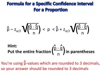
Estimating with confidence - critical z • The z of 1.96 was the z to get a 95% confidence interval. 1.96 is called the critical z, or z*. .025 .475 .475 .025 x .025 is the area to the right of the critical z = 1.96. Let’s call this area to the right of the critical z the upper p critical value.
Here is a summary of some info. Confidence level confidence coefficient alpha z for alpha/2 90% .9 .1 1.645 95% .95 .05 1.96 99% .99 .01 2.58 Then when we multiply the z by the standard error we get the margin of error that is the basis for the confidence interval. The same rules apply for the confidence interval for a population proportion.
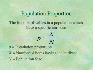
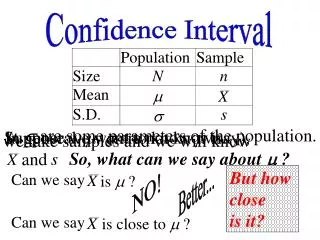
You may recall from a few sections back a company wanted to know if employees participated in a management training program. The sample proportion who said yes is a point estimate of the population proportion. But, we know there is sampling variability, meaning that if we had a different sample we would likely get a different sample proportion. Moreover, the sample proportion is not likely to exactly equal the population proportion. Thus we want to place an interval around the sample proportion in the hopes that the interval will include the population proportion. We will shoot for a certain level of confidence in the interval including the unknown population proportion
Overview • In a previous section we saw the sampling distribution of sample proportions • 1) has a normal distribution • 2) has the same mean as the population proportion from which the sample is drawn (even when we do not know the value – it’s the pattern that is the same), and • 3) has a standard error equal the square root of [π(1-π)]/n. Now in this section for practical purposes we use the sample proportion p in the formula instead of π because we do not know it and are trying to estimate it.
Estimating with confidence - confidence interval To get a 95% confidence interval for the unknown population proportion we 1. Calculate the sample proportion – a point estimate. 2. Take the sample proportion and add 1.96 standard errors. 3. Take the sample proportion and subtract 1.96 standard errors.
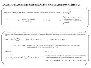
Example: problem 24 page 252 From the information in the problem p = 50/200 = .25. The standard error is sqrt[.25(.75)/200] = .031. A Z of 1.96 will be used with the standard error (multiply the two) to get 1.96(.031) = .06 The confidence interval is then (.19, .31) and we are 95% confident the unknown population proportion is in the interval from .19 to .31.
Problem 26 page 253 a. The sample proportion p = 135/500 = .27 and the standard error is sqrt[.27(.73)/500] = .02. Thus we need to use 2.58 times .02 to get .05. The interval is thus (.22, .32). b. The manager can 99% confident that the unknown proportion of the population will take advantage of the promotion is between .22 and .32. This is less than 1/3 of the population.
Summary In this chapter we have attempted to estimate unknown population parameters. Because we know about sampling variability we build a confidence interval around our point estimate. We have worked on three ideas: 1) Estimate unknown population mean when the population standard deviation is known. We utilize the Z table here. 2) Estimate unknown population mean when the population standard deviation is NOT known. We utilize the t table here. 3) Estimate unknown population proportion. We utilize the Z table here.