Download

1 / 43
430 likes | 512 Views
C ovariate- a djusted M atrix V isualization via C orrelation D ecomposition. 吳漢銘 淡江大學 數學系 資料科學與數理統計組 hmwu@mail.tku.edu.tw http://www.hmwu.idv.tw. Outlines. D ata/Information Visualization T wo Demo Data Sets G eneralized Association Plots ( GAP )

E N D
Covariate-adjusted Matrix Visualizationvia Correlation Decomposition 吳漢銘 淡江大學 數學系 資料科學與數理統計組 hmwu@mail.tku.edu.tw http://www.hmwu.idv.tw
Outlines • Data/Information Visualization • Two Demo Data Sets • Generalized Association Plots (GAP) • Related Works with Matrix Visualization • Covariate-adjusted Matrix Visualization • For a discrete covariate: Within And Between Analysis (WABA) • For a continuous covariate: Partial Correlations • Examples • GAP Software • Concluding Remarks
Data/Information Visualization • Exploiting the human visual system to extract information from data. • Provides an overview of complex data sets. • Identifies structure, patterns, trends, anomalies, and relationships in data. • Assists in identifying the areas of interest. Data information Visualization = Graphing for Data + Fitting + Graphing for Model Matrix Visualization: reorderable matrix, the heatmap, color histogram, data image. Raw Data Matrix Raw Data Map
The Iris Data (Anderson 1935; Fisher 1936) • The iris data published by Fisher (1936) have been widely used for examples in discriminant analysis and cluster analysis. 1 covariate 4 variables setosa Raw Data Matrix 50x3=150 subjects versicolor virginica Images source: http://www.stat.auckland.ac.nz/~ihaka/120/Lectures/lecture27.pdf
Psychosis Disorder Data (Chen 2002) Scale for Assessment of Positive Symptoms (SAPS): 30 items, 4 subgroups. Scale for Assessment of Negative Symptoms (SANS): 20 items, 5 subgroups. Expression (NA1-7) 表達 幻覺 Hallucinations (AH1-6) Speech (NB1-4) 語言 行為 Behavior (BE1-4) Hygiene (NC1-3) 衛生 妄想 Delusions (DL1-12) Activity (ND1-4) 社交 正性症狀: 行為的過量 負性症狀: 行為的不足 Thought disorder (TH1-8) Inattentiveness (NE1-2) 思考失序 做事的意志 All the symptoms are recorded on a six point scale (0-5). 50 Variables 69 schizophrenic 95 Subjects 精神分裂症 精神疾病 26 bipolar disorders Raw Data Matrix 躁鬱症 胡海國 國立臺灣大學 精神科教授 國立臺灣大學醫學院附設醫院 精神部主任
Generalized Association Plots (GAP) (Chen, 2002) Four Steps of Generalized Association Plots (GAP) Proximity Matrices for Rows and Columns Raw Data Matrix Clustering Summarization (1)Presentation呈現 (2) Seriation排序 (3) Partition 分割 (4) Sufficient 充分
Presentation of Raw Data Matrix 0. Data Transformation 1. Selection of Proximity Measures 2. Color Spectrum 3. Display Conditions The 1st Step of GAP
Presentation of Raw Data Matrix: iris data (1) Selection of Proximity Measures Pearson Correlation Matrix for Variables Eculidean Distance Matrix for Subjects (2) Color Spectrum (3) Range Matrix Condition
Presentation of Raw Data Matrix: Psychosis Disorder Data (1) Selection of Proximity Measures Correlation Matrix for Variables Pearson Correlation Coefficient Correlation Matrix for Subjects (2) Color Spectrum Raw Data Matrix (3) Range Matrix Condition
Seriation of Proximity Matrices and Raw Data Matrix • Relativity of a Statistical Graph • Global Criterion • GAP Rank-Two Elliptical Seriation • Local Criterion • Tree Seriation • Flipping of Tree Intermediate Nodes The 2nd Step of GAP
Relativity of a Statistical Graph Placing similar objects at closer positions. Placing different objects at distant positions. Seriation Methods (1) Rank Two Ellipse Ordering (Chen, 2002) Seriation Methods (2) Hierarchical Clustering Tree (Average-Linkage)
GAP Rank-Two Elliptical Seriation Seriation Algorithms with Converging Correlation Matrices Correlation Matrix (without ordering) The p objects fall on an ellipse and have unique relative position on the ellipse (Chen 2002). First two Eigenvectors
ideal model many flips 1 flip 3 flips 5 flips Hierarchical Clustering Tree with a Dendrogram Tree seriation Tree seriation for proximity matrices Different Seriations Generated from Identical Tree Structure Tree seriation for raw data matrices • Internal Tree Flips • External Tree Flips • Ziv Bar-Joseph, David K. Gifford, and Tommi S. Jaakkola, (2001), Fast Optimal Leaf Ordering for Hierarchical Clustering. Bioinformatics 17(Suppl. 1):S22–S29.
Global vs. Local Seriation Data: 517 genes by 13 arrays Michael Eisen (1998) tree seriation GAP Rank-two elliptical seriation Tien, Y. J., Lee, Y. S, Wu, H. M. and Chen, C. H.* (2008), Methods for Simultaneously Identifying Coherent Local Clusters with Smooth Global Patterns in Gene Expression Profiles. BMC Bioinformatics 9:155, 1-16.
Related Works of Matrix Visualization Concept: 1. Bertin (1967): reorderable matrix. 2. Carmichael and Sneath (1969): taxometric maps. Clustering of data arrays: 1. Hartigan (1972): direct clustering of a data matrix. 2. Tibshirani (1999): block clustering. 3. Lenstra (1974): traveling-salesman problem. 4. Slagle et al. (1975): shortest spanning path. Colour Representation: 1. Wegman (1990): colour histogram. 2. Minnotte and West (1998): data image. 3. Marchette and Solka (2003): outlier detection. 1 1 2 1 2 3
Related Works of MV (conti.) 2 Exploring proximity matrices only: 1. Ling (1973): shaded correlation matrix. 2. Murdoch and Chow (1996): elliptical glyphs. 3. Friendly (2002): corrgrams. Integration of raw data matrix with two proximity matrices 1. Chen (1996, 1999, and 2002): generalized association plots (GAP). Reordering of variables and samples 1. Chen (2002): concept of relativity of a statistical graph. 2. Friendly and Kwan (2003): effect ordering of data displays. 3. Hurley (2004): placing interesting displays in prominent positions. Matrix Visualization (MV): reorderable matrix, the heatmap, color histogram, data image. 3 1 1
Covariate-adjusted First two PCAs for Iris Data Psychosis Disorder Data
Covariate-adjusted MV for Discrete Case Correlation (Distance) for rows based on (1) raw data matrix (2) fitted data matrix (3) residual data matrix Correlations for columns Discrete Covariate Y
Within And Between Analysis Dansereau, F., Alutto, J. A., & Yammarino, F. J. (1984). WABA equation Total correlation Between component Within component Between-group correlation Within-group correlation Between-eta correlation Within-eta correlation
Three Steps to WABA WABA I: Assessment of Variation: eta • Each variable is assessed to determine whether the variable varies • between group (suggesting within-group homogeneity). • within groups (suggesting within-group heterogeneity). • both between and within groups (suggesting individual differences rather than within-group homogeneity or heterogeneity).
Three Steps to WABA (conti.) WABA II: Assessment of Covariation: RB, RW • Relationship among variables are assessed to determine whether the correlation between variables is primarily a function of • between-group covariance • within-group covariance • within- and between-group covariance (suggesting individual differences). Drawing Inferences: Combination of WABA I and WABA II: R, B, W • The results of the first two steps are assessed for consistency and combined to draw the best overall conclusion from the data.
Covariate-adjusted MV for Continuous Case Correlations for columns Correlation (Distance) for rows based on (1) raw data matrix (2) fitted data matrix (3) residual data matrix Continuous Covariate Y
Conditional correlation is equivalent to partial correlation under some assumptions (Kurowicka and Cooke, 2000). Partial Correlations
Significance Analysis of the Residual Component • Dunn and Clark’s z test for the equality of two dependent correlations in the case of N exceeds 20 (Steiger, 1980). • Test whether the correlations between variables Xj and Xk are different significantly before andafter a covariate adjustment.
z-scoreSignificant Map • This z-score significant map is helpful identifying variable pairs with the most significant differences in correlation before and after a covariate adjustment. z R R adj Dunn and Clark’s z test
Psychosis Disorder Data: R Rank-two ellipse ordering Five symptom groups identified by Chen (2002). thought disorder (思考失序) Negative (負性症狀) auditory hallucination (聽幻覺) loss of ego boundary (分際喪失) Mania (狂躁) NOTE: the mania symptoms are negatively related to the negative symptoms and the auditory hallucination symptoms.
Psychosis Disorder Data: R=B+W By comparing B and R, the negative correlations between the mania symptoms V5 (DL4, TH6-8) with the negative symptoms V2 (NC1-ND4) and the auditory hallucination symptoms V3 are mostly due to the patients‘ subtypes.
Psychosis Disorder Data: B Average-linkage + GrandPa Flip Delusions (妄想) auditory hallucination symptoms negative symptoms (NC1-ND4) mania symptoms (DL4, TH6-8)
Psychosis Disorder Data: RB Average-linkage + GrandPa Flip • All correlations are either positive one or negative one since there are only two subtypes for patients. • Two clusters (DL2-TH6) and (NA7-NA6) are formed and are negatively correlated. • For 50 between-eta correlations, symptom TH6 with the darkest between-eta has the most significant difference between schizophrenic and bipolar disorders. 話停不下來的 (Pressure of Speech)
Psychosis Disorder Data: W • Rank-two ellipse ordering • Residual Patterns
Psychosis Disorder Data: RW Rank-two ellipse ordering Four new symptom groups: (ND2-NE1), (TH5-TH7), (Th3-Th4) and (DL4-DL6). • Four symptoms NE1, DL2, BE1, and BE2 were grouped into the original negative symptoms group. • The symptoms in the TH (thought disorder) were grouped into two highly correlated subgroups (TH3-TH4, Th5-TH7). • All hallucination symptoms (AH1-6) and most of the delusion symptoms (except DL2, DL3) were clustered together. negative symptoms thought disorder hallucination delusion
Psychosis Disorder Data: Z Positive z scores: • between and within the group of the negative symptoms (V2, except NA6, DL3, and BE4) and the group of the auditory hallucination symptoms (V3, except DL6) • within the group of the mania symptoms (V5, except DL5 and BE3) Negative z scores: • between the group of mania symptoms V5 and the group of the negative symptoms (V2, except DL3, and BE4) and the group of the auditory hallucination symptoms (V3, except DL6). negative auditory hallucination mania
Psychosis Disorder Data: Z Changed significantly: • the symptom TH4 (不合邏輯) of V1 to the group of the negative symptoms (V2, except NA6, DL3, and BE4), the group of the auditory hallucination symptoms (V3, except DL6). Without significant relationship with any other symptom for different patients' subtypes: • Eleven symptoms(TH5, NE2, DL2, BE1, BE2, DL3, BE4, AH6, AH5, DL5,and BE3) • Note: positive symptoms of behavior (BE1-BE4) are all included. thought disorder loss of ego boundary
Psychosis Disorder Data: Z Single-linkage+GrandPa Flip Most significant difference • A right slash: • A reversed slash: • (AH1, DL4), (AH1, TH7), (DL1, DL4), (TH6, NC2), (TH7, NA1), (TH7, NA2), (TH7, NA3) (TH7, NA4), (TH7, NA5), (TH7, NB1), and (TH7, ND1). • Bipolar disorders patients tend to have higher distractible speech score (TH7). • Schizophrenic patients are more likely having higher negative symptoms scores.
Psychosis Disorder Data: Z Single-linkage+GrandPa Flip Most significant difference • A right slash: • A reversed slash: • (AH1, NA5), (DL1, NA4), (DL7, NA1) and (DL7, NA5). • Bipolar disorders patients have lower scores on these symptoms than schizophrenic patients.
Generalized Association Plots Input Data Type: continuous or binary. Various seriation algorithms and clustering analysis. Various display conditions. Modules: Covaraite Adjusted. Proximity Modelling. Nonlinear Association Analysis. Missing Value Imputation. GAP Software verison 0.2.7 • Statistical Plots • 2D Scatterplot, 3D Scatterplot (Rotatable) • Download http://gap.stat.sinica.edu.tw/Software/GAP Wu, H. M., Tien, Y. J. and Chen, C. H.* (2010). GAP: A Graphical Environment for Matrix Visualization and Cluster Analysis, Computational Statistics and Data Analysis, 54, 767-778.
Concluding Remarks Matrix Visualization • Color order-based representation of data matrices. • Provide several levels of information. Covariate-adjusted Matrix Visualization • Decomposition of correlations. • Working on fitted and residual data matrix. • Interactive Software: GAP. • Extension to multi-level data. Suggestions • A preliminary step in modern exploratory data analysis. • A continuing and active topic of research and application. • New generation of exploratory data analysis (EDA) tool. GAP
Acknowledgment hmwu@mail.tku.edu.tw http://www.hmwu.idv.tw cchen@stat.sinica.edu.twhttp://gap.stat.sinica.edu.tw