Download
1 / 56
570 likes | 844 Views
Geospatial Stream Flow Model (GeoSFM). USGS FEWS NET EROS Data Center Sioux Falls, SD 57198. U.S. Department of the Interior U.S. Geological Survey. Objectives. To develop a model for wide-area flood hazard monitoring using existing geospatial datasets

E N D
Geospatial Stream Flow Model(GeoSFM) USGS FEWS NET EROS Data Center Sioux Falls, SD 57198 U.S. Department of the Interior U.S. Geological Survey
Objectives • To develop a model for wide-area flood hazard monitoring using existing geospatial datasets • To use the model to routinely monitor flood hazards across Africa and provide early warning to decision makers
GIS IN FLOOD MONITORING • The Mid-West Floods of 1993 – SAST Database • Creation of Global Elevation Datasets for hydrologic modeling in 1997 • Initiation of GIS-based distributed flood modeling at the USGS in the late 1990s; • Now being applied in Southern Africa, East African and proposed for Mekong River tributaries
ModelOverview • Leverage the vast geospatial data archived at EDC • Initial parameters derived from existing datasets • Input data generated daily from available datasets • Catchment scale modeling framework • Semi-distributed hydrologic model • Inputs aggregated to the catchment level • GIS based Modeling • Takes advantage of existing spatial analysis algorithms • Includes integration with external routing codes
Stream Flow Model GIS Preprocessing GIS Postprocessing Satellite Rainfall Estimates Water Balance Rainfall Forecasts GDAS PET Fields Lumped Routing FAO Soil Data Flood Inundation Mapping Dist. Routing Land Use/ Land Cover Elevation Data Stage Forecasting FEWS Flood Risk Monitoring System Flow Diagram http:/www.fews.net
Geospatial Stream Flow Model, An ArcView 3.2 Extension
Using Menus,Message Boxes and Tools Hydrograph plotting tool Tool for Dam Insertion
Model Components • Terrain Analysis Module • Parameter Estimation Module • Data Preprocessing Module • Water Balance Module • Flow routing Module • Post-processing Module
The goal of Terrain Analysis • to divide the study area into smaller subbasin, rivers • to establish the connectivity between these elements • to compute topography dependent parameters
Flow Direction Flow Accumulation Flow Length Hill Length Slope Subbasins Downstream Subbasin Using ArcView’s Terrain Analysis Functions with USGS 1 km DEM
Key Lessons from Terrain Analysis • Procedures for Terrain Analysis have been refined over the last decade, and they work very well • USGS 1km DEM (Hydro1k) is sufficient for delineation in most basins; it is currently being refined for trouble areas
The goal of Parameter Estimation • to estimate surface runoff parameters in subbasins • to estimate flow velocity and attenuation parameters • to summarize parameters for each subbasin
Estimating Surface Runoff Characteristics • Initially computed on a cell by cell basis • Now moving towards generalizing land cover and soil class over subbasin first (Maidment (Ed.), 1993, Handbook of Hydrology) (Chow et al, 1988, Applied Hydrology)
Overland Velocity with Manning’s Equation • Initially computed on a cell by cell basis • Now moving towards generalizing land cover and slopes class over subbasin first V = (1/n) * R2/3 * S1/2
Weighted flow length and aggregation algorithm to create Unit Hydrographs Overland Velocity, Flow Time Aggregate cells at basin outlet During each routing interval Flow Path, Flow Length
Key Lessons in Parameterization • While GIS routines work well, existing parameter tables in hydrology textbooks are only of limited utility • There is no on-going effort to document parameters from previous studies though these are often extremely useful • Uniform parameter estimates are often at least as good spatially distributed parameters; simpler is better • Field observations and local estimates are invaluable
The goal of Data Processing • to convert available station & satellite rainfall estimates into a common format • to set up ascii files for water balance and flow routing models to ingest
Interpolation routines to grid point rainfall data Grids adhere to a naming convention which allows for subsequent automation Gage Data Daily Grids
Zonal algorithms to compute subbasin mean values and export to an ASCII files Rain / Evap Grid Output to ASCII File Subbasins
Key Lessons in Data Preprocessing • Using a single rainfall value for each subbasin is consistent with the resolution/precision of the satellite rainfall estimates • Saving data values in ASCII files (instead of directly assessing the grids) speeds up subsequent flow routing computations considerably
The goal of Water Balance • to separate input rainfall into evapotranspiration, surface, interflow, baseflow and ground water components • to maintain an accounting of water in storage (soil moisture content) at the end of each simulation time step
Two Water Balance Options • Single layered soil with • “Hortonian” bucket with partial contributing areas • Single subsurface reservoir but different residence times for interflow and baseflow • Two layered soil with • SCS Curve Number Method • Separate reservoirs and residence times for interflow and baseflow
Partitioning Fluxes in single layered model Rainfall Hortonian with Partial Contributing Areas Soil layer Saturated Hydraulic Conductivity Ground Water
Transferring Fluxes in single layered model Rainfall Surface Runoff Unit Hydrograph Soil layer Interflow Linear Reservoir + Baseflow Linear Reservoir Ground Water
Partitioning Fluxes in two layered model Rainfall SCS Curve Number Method Upper layer Lower layer Green – Ampt Based Parameterization Ground Water
Transferring Fluxes in two layered model Rainfall Surface Runoff Unit Hydrograph Upper layer Interflow Conceptual Linear Reservoir Lower layer Baseflow Conceptual Linear Reservoir Ground Water
Key Lessons in Water Balance • SCS Curve number classes don’t correspond directly with mapped land cover / vegetation classes • Hortonian with partial areas performs at least as well and is easier to parameterize than SCS method for runoff generation • Recession portion of the hydrograph has been the most difficult to model correctly
The goal of Flow Routing • to aggregate the runoff contributions of each subbasin at the subbasin outlet • to move the runoff from one subbasin to the next, through the river network to the basin outlet
Within subbasin routing Apply unit hydrograph to excess runoff to obtain runoff at subbasin outlet Runoff Water Balance Unit Hydrograph
Sub-basin 1 Sub-basin 2 + Main channel + Sub-basin 3 Sub-basin 4 Main channel + Outlet Channel Routing Overview
Three Channel Routing Options • Pure Translation Routing • Diffusion Analog Routing • Muskingum Cunge Routing
Pure Translation Routing • Only parameter required is lag time or celerity • Simple but surprising effective in large basins Input Output Flow Flow Time Time
Diffusion Analog Routing • Linear routing method • Requires two parameters • Velocity for translation • Diffusion coefficient for attenuation Input Output Flow Flow Time Time
Muskingum-Cunge Routing Non-Linear, Variable Parameter routing method Accounts for both translation and dispersion River reach Conceptual reach sections with time varying storage Flow Depth Distance along river reach
Key Lessons in Flow Routing • The fewer parameters you have to estimate, the easier it is to obtain a representative model • The ease of developing a representative model often determines readiness of users adopt the model as much as precision of the model • Recommend the diffusion analog model for large scale applications; it achieves a reasonable balance between simplicity and process representation
The goal of Postprocessing • to compute flow statistics (max, min, mean, 25, 75, 33, 66 and 50 percentile flow) • to rank and display current flows relative to percentile flows (high, low, medium) • to perform preliminary inundation mapping (based on uniform flow depths within each reach) • to display hydrographs where needed
Characterizing Flood Risk Produce a synthetic streamflow record Generate Daily Historical Rainfall (1961-96) by reanalysis Determine locations where bankfull storage Is exceeded Compute Bankfull storage