Download
1 / 14
140 likes | 242 Views
5. The Discovery of Production and Its Technology. so far only exchange of goods that can just be gathered now production is discovered, i.e. transformation of existing goods, inputs , into new goods, outputs 5.1 Discovering Production one agent discovers production

E N D
5. The Discovery of Production and Its Technology • so far only exchange of goods that can just be gathered • now production is discovered, i.e. transformation of existing goods, inputs, into new goods, outputs 5.1 Discovering Production one agent discovers production she realizes that others would be willing to pay for the outputs and that by working with others to provide her with inputs they can all be better off than by simply trading the inputs engaging in production implies that other possible activities are foregone, these are the opportunity costs of production normal profit: return that is just sufficient to recover entrepreneur’s opportunity costs anything above is extra-normal profit
5.2 The Production Function and Technology inputs can be combined into outputs only in certain ways technology is a set of constraints on production parallel: preferences are a constraint on the production of utility through consumption goods like utility function can be derived from preferences, production function can be derived from technology assumptions: • No free lunch: No output without input • Nonreversibility: production process cannot be reversed • Free disposability: if one output can be produced with certain inputs, with the same inputs one can produce less • additivity: if x and y can be produced then x+y can • divisibility: if z can be produced, then az, 0<a<1 can • convexity: if v and w can be used to produce z, then one can also use av+(1-a)w to produce z
production function summarizes technology by describing maximal amount of output that can be produced with given input e.g. two inputs: Output = f (input1,input2) As utility function can be represented by set of indifference curves, production function can be represented by a set of isoquants, that describe all input combinations that yield the same output (Fig 5.1) Difference: associated numbers of isoquants have meaning, namely the number of output units
5.3 The Marginal Rate of Technical Substitution marginal rate of technical substitution is (-1 times) the slope of the isoquant, i.e. the rate at which we can substitute one input for the other leaving output fixed marginal product of a factor of production (input) measures change of output if this input is increased by one unit with all other inputs constant (Fig 5.2) MP of input x2 = (change in output) / (change in x2) = y / x2 ratio of MP’s is the slope of isoquant, hence MRTS of x2 for x1 = MP of x1 / MP of x2 = (y/x1) / (y/x2)
5.4 Describing Technologies returns to scale measure how output changes when all inputs are multiplied by the same factor constant RtS: if we double all inputs, output doubles, f(ax1,ax2) = af(x1, x2), e.g. f(K,L) =K1/2L1/2 increasing RtS: if we double all inputs, output more than doubles, f(ax1, ax2) > af(x1, x2) for a>1, e.g. f(K,L) =KL decreasing RtS: if we double all inputs, output less than doubles, f(ax1, ax2) < af(x1, x2) for a>1, f(K,L) =K1/4L1/4 if a technology has constant (or increasing, or decreasing) RtS, then this holds for all its processes, i.e. all efficient input combinations reasons for increasing RtS: specialization of workers, special machines or computerized techniques become efficient if there are increasing RtS then it is better to produce in one factory than in several factories
5.5 Time Constraints to determine optimal combination of input factors, need to know which of these can be varied at all in the immediate run none of the inputs can be varied in the short run there is at least one fixed factor of production, that cannot be varied while there are also variable factors of production that can be varied in the long run all factors are variable long-run production function relates inputs to outputs when all are variable, short-run production function takes one factor as fixed, can be represented in total product curve, relating variable input to output (Fig 5.6) this reflects decreasing returns to factor, i.e. that, holding the other factor (here capital) fixed, additional units of the variable factor (here labor) yield less and less additional output (this does NOT imply decreasing returns to scale) slope of total product curve is marginal prod. curve (Fig 5.7)
6. Cost and Choice assumption: to maximize profits, producer wants to produce at lowest possible costs 6.1 How Costs Are Related to Output cost function describes cheapest (efficient) way to produce a given output ex: no substitution possible, labor and capital have to be used in fixed proportions, constant RtS, (Fig 6.1) • cheapest way to produce hence requires only finding the cheapest way to obtain the capital good • since wages for worker are lower than opportunity costs, hire worker to make capital good • constant returns to scale, no substitution, hence cost function is straight line
optimal (i.e. cost-minimizing) combination of inputs with substitution possibilities • depends on time available for adjustment • in long run, all factors are variable, so can change optimal combination • in short run, at least one factor is fixed, so can only choose the cheapest way to produce for the given level of fixed factors isoquants show different combination of inputs that can be combined in given output the cheapest combination obviously depends on the relative prices of the inputs isocost curves depict combinations of inputs with same costs, slope equals price ratio (relative costs) of inputs optimal combination is the one where isoquant (for desired output) is tangent to (lowest) isocost curve (Fig 6.5)
slope of isoquant is MRTS, slope of isocost curve price ratio hence for optimal combination MRTScapital/labor = MPlabor / MPcapital = wlabor / wcapital if this condition does not hold, producer can substitute one input for the other at different rate than price ratio and hence find a cheaper combination for the same output curve through tangency points (cheapest input combinations for different outputs) is called output expansion path cost function is image of output expansion path in cost-output diagram (Fig 6.6) in the short run optimal input combination is found by using the smallest possible amounts of variable factors to produce desired output in this case isoquant is in general not tangent to isocost curve, producer would like to choose different combination but cannot (Fig 6.7) hence costs in short run at least as high as costs in long run
6.2 Special Technologies and Their Cost Functions The Loentief Technology • inputs have to be used in fixed proportions, e.g. 6 units of labor and 1 unit of capital for 1 unit of output • the corresponding Leontief production function is y=min( labor, 1 capital) • constant returns to scale, no substitution possible • MRTS is either 0 or , hence in optimal combination A we cannot have MRTScapital/labor = wlabor/wcapital • but still A is the point on isoquant that lies on the lowest isocost curve and there (Fig 6.9) MRTSright of A < wlabor/wcapital <MRTSleft of A • cost function is straight line due to constant returns to scale
The Cobb-Douglas Technology • in contrast to Leontief, Cobb –Douglas production function allows for substitution y = K (xcapital) (xlabor) • e.g. K=2, =1/2, =1/2 then choosing xc=1, xl=9, or xc=9, xl=1, or xc=3, xl=3 all yield the same output 6 K ( xcapital) ( xlabor) = +K (xcapital) (xlabor) • hence when + = 1, we have constant returns to scale, CRS-production function, linear cost curve, (Fig 6.12) • when + > 1, we have increasing RtS, concave cost curve • when + < 1, we have decreasing RtS, convex cost curve • Cobb-Douglas function is homothetic, i.e. if all inputs are multiplied by , the output is multiplied by a function of • specifically it is homogenous (i.e. output is multiplied by a power of ) of degree +
if relative prices change, producer will like to change combination of inputs if technology permits this (unlike Leontief) Elasticity of Substitution measures how easily inputs can be substituted if relative prices change: percentage change of ratio of inputs for given percentage change of price ratio, i.e. for k = xc / xl, and w = wc / wl = (k/k) / (w/w) for a Cobb-Douglas production function, the elasticity of substitution is 1, i.e. if the relative prices change by 1%, the ratio of inputs will change by 1% this is so, because for a Cobb-Douglas production function, in the optimal combination of inputs, the ratio of total expenditures for the inputs is constant /
6.3 Short-Run and Long-Run Cost Functions in the short run, when one factor cannot be varied, the costs for this factor are fixed costs, i.e. do not change with level of output, whereas costs for variable factors are variable costs, i.e. change with level of output in the long run all costs are variable short-run total cost function shows the total cost of producing output, starts with fixed costs for an output level of 0. (Fig 6.15) short-run average cost function shows the short-run cost per unit of output, corresponds to slope of line from origin to point on total cost function short-run marginal cost function is the slope of the short-run total cost function average cost is minimized where it is equal to marginal cost average total cost = average fixed cost(falling) + average variable cost (U-shape due to diminishing returns to the variable factor)
in short run, for each level of the fixed factor capital there is a set of short-run total, average and marginal cost functions • for known level of output capital, hence fixed-costs will be chosen optimally, i.e. less for smaller levels of output • ex: three possible levels of capital (Fig 6.18) optimal level of capital is the level of capital of the lowest average (and hence lowest total) cost curve hence long-run average (or total) cost curve is the lower boundary of the family of short-run average (or total) cost curves (in the long run, we can always choose capital optimally and will hence choose the level such that average, and hence total, cost is minimal) long-run marginal cost = short-run marginal cost where long-run average cost = short-run average cost (Fig 6.20) long-run average costs are minimal where they are equal to long-run marginal costs