Download
1 / 40
400 likes | 501 Views
Uncalibrated Camera. Lecture 5 Uncalibrated Geometry & Stratification. calibrated coordinates. Linear transformation. pixel coordinates. Uncalibrated Camera. Calibration with a rig Uncalibrated epipolar geometry Ambiguities in image formation Stratified reconstruction

E N D
Uncalibrated Camera Lecture 5Uncalibrated Geometry & Stratification Invitation to 3D vision
calibrated coordinates Linear transformation pixel coordinates Uncalibrated Camera Invitation to 3D vision
Calibration with a rig Uncalibrated epipolar geometry Ambiguities in image formation Stratified reconstruction Autocalibration with partial scene knowledge Overview Invitation to 3D vision
Calibrated camera • Image plane coordinates • Camera extrinsic parameters • Perspective projection Uncalibrated camera • Pixel coordinates • Projection matrix Uncalibrated Camera Invitation to 3D vision
Taxonomy on Uncalibrated Reconstruction • is known, back to calibrated case • is unknown • Calibration with complete scene knowledge (a rig) – estimate • Uncalibrated reconstruction despite the lack of knowledge of • Autocalibration (recover from uncalibrated images) • Use partial knowledge • Parallel lines, vanishing points, planar motion, constant intrinsic • Ambiguities, stratification (multiple views) Invitation to 3D vision
Calibration with a Rig Use the fact that both 3-D and 2-D coordinates of feature points on a pre-fabricated object (e.g., a cube) are known. Invitation to 3D vision
Given 3-D coordinates on known object • Eliminate unknown scales • Solve for translation Calibration with a Rig • Recover projection matrix • Factor the into and using QR decomposition Invitation to 3D vision
Epipolar constraint • Fundamental matrix • Equivalent forms of Uncalibrated Epipolar Geometry Invitation to 3D vision
Properties of the Fundamental Matrix • Epipolar lines • Epipoles Image correspondences Invitation to 3D vision
Properties of the Fundamental Matrix A nonzero matrix is a fundamental matrix if has a singular value decomposition (SVD) with for some . There is little structure in the matrix except that Invitation to 3D vision
Estimating Fundamental Matrix • Find such Fthat the epipolar error is minimized Pixel coordinates • Fundamental matrix can be estimated up to scale • Denote • Rewrite • Collect constraints from all points Invitation to 3D vision
Two view linear algorithm – 8-point algorithm • Solve the LLSEproblem: • Solution eigenvector associated with • smallest eigenvalue of • Compute SVD of F recovered from data • Projectonto the essential manifold: • cannot be unambiguously decomposed into pose • and calibration Invitation to 3D vision
Calibrated vs. Uncalibrated Space Invitation to 3D vision
Calibrated vs. Uncalibrated Space Distances and angles are modified by S Invitation to 3D vision
Motion in the distorted space Calibrated space Uncalibrated space • Uncalibrated coordinates are related by • Conjugate of the Euclidean group Invitation to 3D vision
can be inferred from point matches (eight-point algorithm) Cannot extract motion, structure and calibration from one fundamental matrix (two views) allows reconstruction up to a projective transformation (as we will see soon) encodes all the geometric information among two views when no additional information is available What Does F Tell Us? Invitation to 3D vision
Decomposition of the fundamental matrix into a skew • symmetric matrix and a nonsingular matrix Decomposing the Fundamental Matrix • Decomposition of is not unique • Unknown parameters - ambiguity • Corresponding projection matrix Invitation to 3D vision
Projective Reconstruction • From points, extract , followed by computation of projection matrices and structure • Canonical decomposition • Given projection matrices – recover structure • Projective ambiguity – non-singular 4x4 matrix Both and are consistent with the epipolar geometry – give the same fundamental matrix Invitation to 3D vision
Projective Reconstruction • Given projection matrices recover projective structure • This is a linear problem and can be solve using linear least-squares • Projective reconstruction – projective camera matrices and • projective structure Invitation to 3D vision Projective Structure Euclidean Structure
Euclidean reconstruction – true metric properties of objects lenghts (distances), angles, parallelism are preserved Unchanged under rigid body transformations => Euclidean Geometry – properties of rigid bodies under rigid body transformations, similarity transformation Projective reconstruction – lengths, angles, parallelism are NOT preserved – we get distorted images of objects – their distorted 3D counterparts --> 3D projective reconstruction => Projective Geometry Euclidean vs Projective reconstruction Invitation to 3D vision
Homogeneous coordinates: Homogeneous Coordinates (RBM) 3-D coordinates are related by: Homogeneous coordinates are related by: Invitation to 3D vision
Homogenous and Projective Coordinates • Homogenous coordinates in 3D before – attach 1 as the last coordinate – render the transformation as linear transformation • Projective coordinates – all points are equivalent up to a scale 2D- projective plane 3D- projective space • Each point on the plane is represented by a ray in projective space • Ideal points – last coordinate is 0 – ray parallel to the image plane • points at infinity – never intersects the image plane Invitation to 3D vision
Vanishing points – points at infinity Representation of a 3-D line – in homogeneous coordinates When -> 1 - vanishing points – last coordinate -> 0 Similarly in the image plane Invitation to 3D vision
Ambiguities in the image formation • Potential Ambiguities • Ambiguity in K (K can be recovered uniquely – Cholesky or QR) • Structure of the motion parameters • Just an arbitrary choice of reference frame Invitation to 3D vision
Ambiguities in Image Formation Structure of the (uncalibrated) projection matrix • For any invertible 4 x 4 matrix • In the uncalibrated case we cannot distinguish between camera imaging word from camera imaging distorted world • In general, is of the following form • In order to preserve the choice of the first reference frame we can restrict some DOF of Invitation to 3D vision
Structure of the Projective Ambiguity • 1st frame as reference • Choose the projective reference frame then ambiguity is • can be further decomposed as Invitation to 3D vision
Stratified (Euclidean) Reconstruction • General ambiguity – while preserving choice of first reference frame • Decomposing the ambiguity into affine and projective one • Note the different effect of the 4-th homogeneous coordinate Invitation to 3D vision
Affine upgrade • Upgrade projective structure to an affine structure • Exploit partial scene knowledge • Vanishing points, no skew, known principal point • Special motions • Pure rotation, pure translation, planar motion, rectilinear motion • Constant camera parameters (multi-view) Invitation to 3D vision
Affine upgrade using vanishing points How to compute Maps the points To points with affine coordinates Vanishing points – last homogeneous affine coordinate is 0 Invitation to 3D vision
Affine Upgrade Need at least three vanishing points 3 equations, 4 unknowns (-1 scale) Solve for Set up and update the projective structure Invitation to 3D vision
Euclidean upgrade • We need to estimate remaining affine ambiguity • In the case of special motions (e.g. pure rotation) – no projective ambiguity – cannot do projective reconstruction • Estimate directly (special case of rotating camera – follows) • Multi-view case – estimate projective and affine ambiguity together • Use additional constraints of the scene structure (next) • Autocalibration (Kruppa equations) Alternatives: Invitation to 3D vision
Euclidean Upgrade using vanishing points • Vanishing points – intersections of the parallel lines • Vanishing points of three orthogonal directions • Orthogonal directions – inner product is zero • Provide directly constraints on matrix • S – has 5 degrees of freedom, 3 vanishing points – 3 constraints (need additional assumption about K) • Assume zero skew and aspect ratio = 1 Invitation to 3D vision
Geometric Stratification Invitation to 3D vision
Special Motions – Pure Rotation • Calibrated Two views related by rotation only • Mapping to a reference view – rotation can be estimated • Mapping to a cylindrical surface Invitation to 3D vision
Pure Rotation - Uncalibrated Case • Calibrated Two views related by rotation only • Conjugate rotation can be estimated • Given C, how much does it tell us about K (or S) ? • Given three rotations around linearly independent axes – S, K can be estimated using linear techniques • Applications – image mosaics Invitation to 3D vision
Overview of the methods Invitation to 3D vision
Summary Invitation to 3D vision
Direct Autocalibration Methods The fundamental matrix satisfies the Kruppa’s equations If the fundamental matrix is known up to scale Under special motions, Kruppa’s equations become linear. Solution to Kruppa’s equations is sensitive to noises. Invitation to 3D vision
Direct Stratification from Multiple Views From the recovered projective projection matrix we obtain the absolute quadric contraints Partial knowledge in (e.g. zero skew, square pixel) renders the above constraints linear and easier to solve. The projection matrices can be recovered from the multiple-view rank method to be introduced later. Invitation to 3D vision
Summary of (Auto)calibration Methods Invitation to 3D vision