Download
1 / 65
650 likes | 660 Views
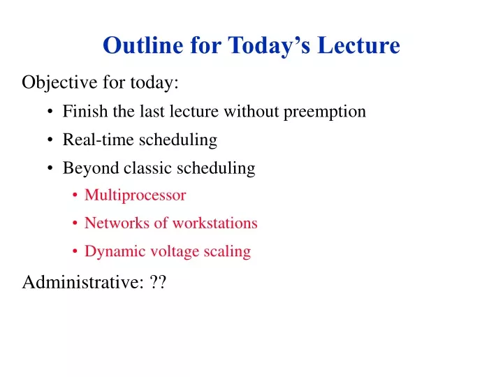
Outline for Today’s Lecture. Objective for today: Finish the last lecture without preemption Real-time scheduling Beyond classic scheduling Multiprocessor Networks of workstations Dynamic voltage scaling Administrative: ??. Preemptive FCFS: Round Robin.

E N D
Outline for Today’s Lecture • Objective for today: • Finish the last lecture without preemption • Real-time scheduling • Beyond classic scheduling • Multiprocessor • Networks of workstations • Dynamic voltage scaling • Administrative: ??
Preemptive FCFS: Round Robin • Preemptive timeslicing is one way to improve fairness of FCFS. • If job does not block or exit, force an involuntary context switch after each quantum Q of CPU time. • Preempted job goes back to the tail of the ready list. • With infinitesimal Q round robin is called processor sharing. D=3 D=2 D=1 FCFS round robin 6 3+ε 5 quantum Q=1 R = (3 + 5 + 6 + ε)/3 = 4.67 + ε In this case, R is unchanged by timeslicing. Is this always true? preemption overhead = ε
Evaluating Round Robin D=5 D=1 • Response time. RR reduces response time for short jobs. • For a given load, a job’s wait time is proportional to its D. • Fairness. RR reduces variance in wait times. • But: RR forces jobs to wait for other jobs that arrived later. • Throughput. RR imposes extra context switch overhead. • CPU is only Q/(Q+ε) as fast as it was before. • Degrades to FCFS with large Q. R = (5+6)/2 = 5.5 R = (2+6 + ε)/2 = 4 + ε Q is typically 5-100 milliseconds; ε is 1-5 μs in 1998.
D=3 D=2 D=1 6 1 3 Minimizing Response Time: SJF • Shortest Job First (SJF) is provably optimal if the goal is to minimize R. • Example: express lanes at the MegaMart • Idea: get short jobs out of the way quickly to minimize the number of jobs waiting while a long job runs. • Intuition: longest jobs do the least possible damage to the wait times of their competitors. R = (1 + 3 + 6)/3 = 3.33
SJF • In preemptive case, shortest remaining time first. • In practice, we have to predict the CPU service times (computation time until next blocking). • Favors interactive jobs, needing response, & repeatedly doing user interaction • Favors jobs experiencing I/O bursts - soon to block, get devices busy, get out of CPU’s way • Focus is on an average performance measure, some long jobs may starve under heavy load/ constant arrival of new short jobs.
Behavior of SJF Scheduling • With SJF, best-case R is not affected by the number of tasks in the system. • Shortest jobs budge to the front of the line. • Worst-case R is unbounded, just like FCFS. • Since the queue is not “fair”, starvation exists - the longest jobs are repeatedly denied the CPU resource while other more recent jobs continue to be fed. • SJF sacrifices fairness to lower average response time.
SJF in Practice • Pure SJF is impractical: scheduler cannot predict D values. • However, SJF has value in real systems: • Many applications execute a sequence of short CPU bursts with I/O in between. • E.g., interactive jobs block repeatedly to accept user input. • Goal: deliver the best response time to the user. • E.g., jobs may go through periods of I/O-intensive activity. • Goal: request next I/O operation ASAP to keep devices busy and deliver the best overall throughput. • Use adaptive internal priority to incorporate SJF into RR. • Weather report strategy: predict future D from the recent past.
start (arrival rate λ) I/O completion I/O request I/O device exit (throughput λ until some center saturates) CPU Considering I/O • In real systems, overall system performance is determined by the interactions of multiple service centers. A queue network has K service centers. Each job makes Vk visits to center k demanding service Sk. Each job’s total demand at center k is Dk = Vk*Sk Forced Flow Law: Uk = λk Sk = λ Dk (Arrivals/throughputs λk at different centers are proportional.) Easy to predict Xk, Uk, λk, Rk and Nk at each center: use Forced Flow Law to predict arrival rate λk at each center k, then apply Little’s Law to k. Then: R = ΣVk*Rk
Digression: Bottlenecks • It is easy to see that the maximum throughput X of a system is reached as 1/λ approaches Dk for service center k with the highest demand Dk. • k is called the bottleneck center • Overall system throughput is limited byλkwhen Uk approaches 1. Example 1: CPU S0 = 1 I/O S1 = 4 This job is I/O bound. How much will performance improve if we double the speed of the CPU? Is it worth it? To improve performance, always attack the bottleneck center! Example 2: CPU S0 = 4 I/O S1 = 4 Demands are evenly balanced. Will multiprogramming improve system throughput in this case?
Two Schedules for CPU/Disk 1. Naive Round Robin 5 1 5 1 4 CPU busy 25/37: U = 67% Disk busy 15/37: U = 40% 2. Round Robin with SJF 33% performance improvement CPU busy 25/25: U = 100% Disk busy 15/25: U = 60%
high low Multilevel Feedback Queue • Many systems (e.g., Unix variants) implement priority and incorporate SJF by using a multilevel feedback queue. • multilevel. Separate queue for each of N priority levels. • Use RR on each queue; look at queue i-1 only if queue i is empty. • feedback. Factor previous behavior into new job priority. I/O bound jobs waiting for CPU jobs holding resouces jobs with high external priority GetNextToRun selects job at the head of the highest priority queue. constant time, no sorting CPU-bound jobs Priority of CPU-bound jobs decays with system load and service received. ready queues indexed by priority
Real Time Schedulers • Real-time schedulers must support regular, periodic execution of tasks (e.g., continuous media). • e.g. Microsoft’s Rialto scheduler [Jones97] supports an external interface for: • CPU Reservations • “I need to execute for X out of every Y units.” • Scheduler exercises admission control at reservation time: application must handle failure of a reservation request. • Time Constraints • “Run this before my deadline at time T.”
Assumptions • Tasks are periodic with constant interval between requests, Ti (request rate 1/Ti) • Each task must be completed before the next request for it occurs • Tasks are independent • Run-time for each task is constant (max), Ci • Any non-periodic tasks are special
Task Model C1 = 1 t1 Ti Ti t2 C2 = 1 T2 time
Definitions • Deadline is time of next request • Overflow at time t if t is deadline of unfulfilled request • Feasible schedule - for a given set of tasks, a scheduling algorithm produces a schedule so no overflow ever occurs. • Critical instant for a task - time at which a request will have largest response time. • Occurs when task is requested simultaneously with all tasks of higher priority
Rate Monotonic • Assign priorities to tasks according to their request rates, independent of run times • Optimal in the sense that no other fixed priority assignment rule can schedule a task set which can not be scheduled by rate monotonic. • If feasible (fixed) priority assignment exists for some task set, rate monotonic is feasible for that task set.
Task Model C1 = 1 t1 T1 T1 t2 C2 = 1 T2 time
Earliest Deadline First • Dynamic algorithm • Priorities are assigned to tasks according to the deadlines of their current request • With EDF there is no idle time prior to an overflow • For a given set of m tasks, EDF is feasible iffC1/T1 + C2/T2 + … + Cm/Tm[ 1 • If a set of tasks can be scheduled by any algorithm, it can be scheduled by EDF
Task Model C1 = 1 t1 T1 T1 t2 C2 = 1 T2 time
t1 t0 Proportional Share • Goals: to integrate real-time and non-real-time tasks, to police ill-behaved tasks, to give every process a well-defined share of the processor. • Each client, i, gets a weight wi • Instantaneous share fi (t) = wi /(S wj ) • Service time (fi constant in interval)Si(t0, t1) = fi (t) Dt • Set of active clients varies ->fi varies over timeSi(t0 , t1) = fi (t) dt jcA(t)
Common Proportional Share Competitors • Weighted Round Robin – RR with quantum times equal to share RR: WRR: • Fair Share –adjustments to priorities to reflect share allocation (compatible with multilevel feedback algorithms) 30 20 20 10 Linux
Common Proportional Share Competitors • Weighted Round Robin – RR with quantum times equal to share RR: WRR: • Fair Share –adjustments to priorities to reflect share allocation (compatible with multilevel feedback algorithms) 20 10 10 10 Linux
Common Proportional Share Competitors • Weighted Round Robin – RR with quantum times equal to share RR: WRR: • Fair Share –adjustments to priorities to reflect share allocation (compatible with multilevel feedback algorithms) 10 0 10 Linux
2/3 2/2 1/1 t Common Proportional Share Competitors • Fair Queuing • Weighted Fair Queuing • Stride scheduling • VT – Virtual Time advances at a rate proportional to share • VFT – Virtual Finishing Time: VT a client would have after executing its next time quantum • WFQ schedules by smallest VFT • EA never below -1 VTA(t) = WA(t) / SA VFT = 3/3VFT = 3/2VFT = 2/1
Lottery Scheduling • Lottery scheduling[Waldspurger96]is another scheduling technique. • Elegant approach to periodic execution, priority, and proportional resource allocation. • Give Wp “lottery tickets” to each process p. • GetNextToRun selects “winning ticket” randomly. • If ΣWp = N, then each process gets CPU share Wp/N ... ...probabilistically, and over a sufficiently long time interval. • Flexible: tickets are transferable to allow application-level adjustment of CPU shares. • Simple, clean, fast. • Random choices are often a simple and efficient way to produce the desired overall behavior (probabilistically).
Example List-based Lottery T = 20 5 2 1 10 2 12 Summing: 10 17 Random(0, 19) = 15
Linux Scheduling Policy • Runnable process with highest priority and timeslice remaining runs (SCHED_OTHER policy) • Dynamically calculated priority • Starts with nice value • Bonus or penalty reflecting whether I/O or compute bound by tracking sleep time vs. runnable time: sleep_avg and decremented by timer tick while running
Linux Scheduling Policy • Dynamically calculated timeslice • The higher the dynamic priority, the longer the timeslice: • Recalculated every round when “expired” and “active” swap • Exceptions for expired interactive • Go back on active unless there are starving expired tasks High prioritymore interactive Low priorityless interactive 10ms 150ms 300ms
Linux task_struct • Process descriptor in kernel memory represents a process (allocated on process creation, deallocated on termination). • Linux: task_struct, located via task pointer in thread_info structure on process’s kernel state. task_struct task_struct stateprio policy static_priosleep_avgtime_slice …
. . . . . . . . . . . . Runqueue for O(1) Scheduler Higher prioritymore I/O 300ms priority array priority queue active lower prioritymore CPU 10ms priority queue expired priority array priority queue priority queue
. . . . . . Runqueue for O(1) Scheduler priority array 0 priority queue 1 . . . active priority queue expired priority array priority queue . . . priority queue
X . . . . . . . . . . . . X Runqueue for O(1) Scheduler priority array 0 priority queue active priority queue expired priority array priority queue 1 priority queue
Linux Real-time • No guarantees • SCHED_FIFO • Static priority, effectively higher than SCHED_OTHER processes* • No timeslice – it runs until it blocks or yields voluntarily • RR within same priority level • SCHED_RR • As above but with a timeslice. * Although their priority number ranges overlap
Beyond “Ordinary” Uniprocessors • Multiprocessors • Co-scheduling and gang scheduling • Hungry puppy task scheduling • Load balancing • Networks of Workstations • Harvesting Idle Resources - remote execution and process migration • Laptops and mobile computers • Power management to extend battery life, scaling processor speed/voltage to tasks at hand, sleep and idle modes.
Multiprocessor Scheduling • What makes the problem different? • Workload consists of parallel programs • Multiple processes or threads, synchronized and communicating • Latency defined as last piece to finish. • Time-sharing and/or Space-sharing (partitioning up the Mp nodes) • Both when and where a process should run
Mem Mem Node 0 Node 1 P P CA CA $ $ Interconnect CA CA $ $ Mem Mem P P Node 3 Node 2 Architectures Symmetric mp NUMA P P P P $ $ $ $ Memory cluster
Affinity Scheduling • Where (on which node) to run a particular thread during the next time slice? • Processor’s POV: favor processes which have some residual state locally (e.g. cache) • What is a useful measure of affinity for deciding this? • Least intervening time or intervening activity (number of processes here since “my” last time) * • Same place as last time “I” ran. • Possible negative effect on load-balance.
Every processor has its own private runqueue Locking – spinlock protects runqueue Load balancing – pulls tasks from busiest runqueue into mine. Affinity – cpus_allowed bitmask constrains a process to particular set of processors load_balance runs from schedule( ) when runqueue is empty or periodically esp. during idle. Prefers to pull processes from expired, not cache-hot, high priority, allowed by affinity Linux Support for SMP Symmetric mp P P P P $ $ $ $ Memory
Processor Partitioning • Static or Dynamic • Process Control (Gupta) • Vary number of processors available • Match number of processes to processors • Adjusts # at runtime. • Works with task-queue or threads programming model • Suspend and resume are responsibility of runtime package of application • Impact on “working set”
Process Control ClaimsTypical speed-up profile Lock contention, memory contention, context switching, cache corruption ||ism and working set in memory speedup Magic point Number of processes per application
Co-Scheduling • John Ousterhout (Medusa OS) • Time-sharing model • Schedule related threads simultaneouslyWhy? • Common state and coordination • How? • Local scheduling decisions after some global initialization (Medusa) • Centralized (SGI IRIX)
Effect of Workload • Impact of communication and cooperation • Issues: • context switch • common state • lock contention • coordination
CM*’s Version • Matrix S (slices) x P (processors) • Allocate a new set of processes (task force) to a row with enough empty slots • Schedule: Round robin through rows of matrix • If during a time slice, this processor’s element is empty or not ready, run some other task force’s entry in this column - backward in time (for affinity reasons and purely local “fall-back” decision)
Networks of Workstations • What makes the problem different? • Exploiting otherwise “idle” cycles. • Notion of ownership associated with workstation. • Global truth is harder to come by in wide area context
Harvesting Idle Cycles • Remote execution on an idle processor in a NOW (network of workstations) • Finding the idle machine and starting execution there. Related to load-balancing work. • Vacating the remote workstation when its user returns and it is no longer idle • Process migration
Issues • Why? • Which tasks are candidates for remote execution? • Where to find processing cycles? What does “idle” mean? • When should a task be moved? • How?
Motivation for Cycle Sharing • Load imbalances. Parallel program completion time determined by slowest thread. Speedup limited. • Utilization. In trend from shared mainframe to networks of workstations -> scheduled cycles to statically allocated cycles • “Ownership” model • Heterogeneity
Which Tasks? • Explicit submission to a “batch” scheduler (e.g., Condor) or Transparent to user. • Should be demanding enough to justify overhead of moving elsewhere. Properties? • Proximity of resources. • Example: move query processing to site of database records. • Cache affinity
Finding Destination • Defining “idle” workstations • Keyboard/mouse events? CPU load? • How timely and complete is the load information (given message transit times)? • Global view maintained by some central manager with local daemons reporting status. • Limited negotiation with a few peers • How binding is any offer of free cycles? • Task requirements must match machine capabilities