Download
1 / 35
350 likes | 498 Views
Random (but hopefully useful) STATA commands. Jen Cocohoba, Pharm.D ., MAS Health Sciences Associate Clinical Professor UCSF School of Pharmacy. Housekeeping. Evolution of this lecture “How do I … for my final project/research project” Assortment of topics Data in other formats

E N D
Random (but hopefully useful) STATA commands Jen Cocohoba, Pharm.D., MAS Health Sciences Associate Clinical Professor UCSF School of Pharmacy
Housekeeping • Evolution of this lecture • “How do I … for my final project/research project” • Assortment of topics • Data in other formats • Programming a loop • Managing duplicate observations • Date data in STATA • Basic merging for datasets • Introduction to reshaping data • Follow along • No lab exercises – work on final project
SAS files • Step 1: check your SAS dataset type • STATA can read SAS xport files (*.xpt, *.stx) import sasxport “dataset.xpt” • If you have both SAS and STATA on your computer • Method 1: use SAS to turn it into a STATA dataset • Open dataset in SAS • Menu File Export choose STATA dataset as type • Save the new dataset • Can do this at UCSF library if you don’t own SAS • Method 2: download usesas package • Module requires both programs on computer to “read” sas datasets ssc install usesas, replace usesas using “filename.sasb7dat”
SPSS datasets • Method 1: similar to previous • Open dataset in SPSS and save as STATA dataset • Method 2: usespss • Plugin “reader” installed into STATA which does not require you to have SPSS installed • Type finditusespssto download • Reads *.sav files originating from WINDOWS SPSS usespss using “dataset.sav” For more information: http://adeptanalytics.org/radyakin/stata/usespss/radyakin_usespss.pdf
Programming loops Table 1 • Example • Determine whether age, number of side effects, and scaled severity of side effects differ by gender • Start programming… ttestage, by(sex) ttestnumsidefx, by(sex) ttestseverity, by(sex)
Simple Loop Syntax Loop begin foreach var in variable1 variable2 { firstcommand `var’ secondcommand `var’ } List of variables Perform these commands, replacing the `var’ with the variables in the list. NOTE the special apostrophe marks (the first one lies below the ~ on the keyboard, the other is a normal apostrophe) Loop end • * NOTES • Open brace must appear on the same line as the foreach command. • Nothing may follow the open brace (except for comments) • The first command must be on a separate line • The close brace must be on its own line
Simple Loop Syntax Loop begin foreach var in age numsidefx severity { ttest `var’, by(gender) } Variables Perform this command, replacing the generic placeholder `var’ with variables I specified in my list. NOTE the special apostrophe marks (the first one lies below the ~ on the keyboard, the other is a normal apostrophe) Loop end • * NOTES • Open brace must appear on the same line as the foreach command. • Nothing may follow the open brace (except for comments) • The first command must be on a separate line • The close brace must be on its own line
Loops in do files - examples ******** Frequencies for Table 1 – baseline characteristics ******** /* Get proportions of categorical variables and estimates of missing */ foreachvar in agecatafamerhighschool income employed insurtype{ tab `var' sex, missing col chi2 } /* Get means, standard deviations, and test for differences of continuous variables */ foreach var in ageatvisit cd4 log10vl { bysortsex: sum `var', detail ttest `var', by(sex) } ******** Table 2 Odds Ratios ******** /* Get all of the univariate odds ratios for important factors with guideline not recommended regimens */ foreachvar in highschool income employed drugcover depressed { xi: logistic guideline i.`var' }
Handling Duplicate Observations • Just want to find the duplicates? duplicates list variable1 variable2 Or… duplicates report variable1 variable2 or… duplicates tag variable1 variable2, gen(newvar)
Handling Duplicate Observations Usual goal is to either find the duplicates or get rid of them … or both Method 1: 2 step process of tagging then dropping duplicates tag variable1 variable2, gen(newvar) duplicates drop if newvar==1 Method 2: just dropping duplicates drop variable1 variable2, force
STATA dates • Dates common in research • STATA reads dates as string • Do the “usual” • Open Excel spreadsheet, copy, paste into editor • (OR import the data) • Note color of variable
How STATA thinks about dates 1/1/1960 1/3/1960 12/31/1960 • “Counts” date as the # of days from a specific reference • January 1, 1960 = 0 • January 2, 1960 = 1 • January 3, 1960 = 2 • December 31, 1960 = 364 • This makes it “easy” for STATA to manipulate mathematically • We will come back to this when formatting dates 0 1 2 364
Cleaning STATA dates • Need to convert to STATA-recognizable date to perform analysis • Generate a new date variable using date function • Identify the “old” string variable which contains the date • Tell STATA what format it was in (e.g. month, day, year) • Compare old and new results
generate dob = date(birthdate, “MDY”, topyear) For 2-digit years, the “top year” that should be interpreted New variable name Date function Old variable name How the date is arranged *NOTE: your original date variable can be “date-like” (e.g. 8/10/1970) or can be in a true string format (August 10, 1970) --- STATA can figure it out.
Number nonsense • Emerges as the date in STATA speak • Can mask the numerical date so that it is easier for you to understand Command: format dob %td dob -2372 -4366 -3839 150 -4862 -3626 -2788 -3562 -1868 -5946 -5984 -1962 -4694 -6018 -4407 0 * NOTE: Other formats aside from %td – in STATA help
Dates: series of commands • Date conversions usually 2-commands plus checking generate dob = date(birthdate, “MDY”) format dob %td browse dob birthdate drop birthdate • NOTE: STATA issues with 2-digit years (8/10/76) • Will get “missing values” generated • Two ways to fix this • Format dates to 4 digit years in Excel, then copy to STATA • Add “topyear” cutoff to the STATA command. • Anything beyond topyear = previous century generate dob = date(birthdate, “MDY”, 2012) 9/10/11 = September 10, 2011 9/10/12 = September 10, 2012 top year 9/10/13 = September 10, 1913 9/10/14 = September 10, 1914
MDY command • Date components housed in separate variables New variable name mdy date function • STATA can concatenate these for you Name of month, day, and year variables
Date is now formatted – what can you do with it? • Extract components of the date into new variables (columns) • gen nameofdayvariable = day(datevariable) • gen weekdayvariable = dow(datevariable) • Lists as 0(Sunday) - 6(Saturday) • gen monthvariable = month(datevariable) • gen yearvariable = year(datevariable)
What else can you do with dates • Find time elapsed between dates • Suppose you wanted to find participants’ age at the date of their study visit (or today) • Generate new variable called ageatvisit gen ageatvisit = vdate - dob • Note this gives you their age in number of DAYS • Can do this more efficiently by gen ageatvisit =(vdate – dob)/365.25 gen agevisityears = int(ageatvisit)
Comparing dates • Suppose you wanted to categorize patients by a date • Patients starting ARV < 1996 = pre-HAART • Using literal dates • Formatted as day month year (01jan1960) • Must be denoted by parenthesis • Must use pseudocommandtd • Example: td(01jan1960) • Example • gen prehaart= 0 • replace prehaart= 1 if artstart<= td(01jan2006) • replace prehaart=. if artstart==.
A little on merging datasets • Merge versus append • Merge = add new variables from 2nd dataset to existing obs (across) • Append = add new obs to existing variables (under) • Merging requires datasets to have a common variable (ID) • Nomenclature for the datasets • One dataset is defined as the “master” (in memory) dataset • The other dataset is called the “using” dataset • Many merge types – need to specify for STATA
One to One/One to many • merge 1:1 • merge 1:m master master using using
Many to one, Many to Many • merge m:1 • merge m:m using master master using
Merging datasets • Need to make sure data are sorted by the common variable AND saved • Steps • Load the master dataset into memory • Sort (just to be safe) & save • Merge command • Check to make sure it makes sense sort idvariable merge type commonvariable using “name of 2nd dataset.dta” • See appearance of a “merge” variable which tells you where the observations came from (dataset 1, dataset 2, etc.) Example: with two datasets called “wihsdrugs” (master) and “socdem” (using) use “socdem.dta” sort wihsid save “socdem.dta”, replace clear use “wihsdrugs.dta” sort wihsid merge 1:1 wihsid using “socdem.dta” browse
Shape-shifting • Conceptually difficult • Example: chart with patients and average # cigarettes smoked per day over time WIDE • May want data to look different to manipulate LONG
Reshaping wide to long • Wide to long: make dataset with multiple records per patient • Group variables need common “stub” • In our example 1982, 1983, 1984 • STATA doesn’t know to group these unless named similarly rename 1982 cigs1982 rename 1983 cigs1983 rename 1984 cigs1984 • Nomenclature • i = primary index variable (the patient identification number) • j = secondary index variable (often generated from a “stub”) reshape long cigs, i(idnumber) j(year)* Stub New variable
Reshaping long to wide • Long to wide: one record per patient (our example) reshape wide datavariable, i(indexvariable) j(2nd-indexvar) reshape wide cigs, i(idnumber) j(year) Stub: to be created Existing variable (going to be dropped)
The wonders of STATA • What statistical test do I run… • Google and Statisticians • How do I run a particular test/command … • STATA within-program help feature • STATA help (http://www.stata.com/support) • UCLA STATA site (http://www.ats.ucla.edu/stat/stata) • Google & other web discussion strings • Good luck with your final projects!