Download
1 / 77
770 likes | 885 Views
THE NEURAL-NETWORK ANALYSIS & its applications DATA FILTERS. Saint-Petersburg State University JASS 2006. About me. Name : Alexey Minin Place of studying: Saint-Petersburg State University Current semester: 7 th semester

E N D
THE NEURAL-NETWORK ANALYSIS & its applicationsDATA FILTERS Saint-Petersburg State University JASS 2006
About me Name:Alexey Minin Place of studying:Saint-Petersburg State University Current semester:7th semester Field of interests:Neural Nets, Data filters for Optics (Holography), Computational Physics,EconoPhisics.
Content: • What is Neural Net & it’s applications • Neural Net analysis • Self organizing Kohonen maps • Data filters • Obtained results
What is NeuroNet & it’s applications • Recognition of images • Processing of noised signals • Addition of images • Associative search • Classification • Drawing up of schedules • Optimization • The forecast • Diagnostics • Prediction of risks these are what i am doing
What is Neural Net & it’s applications Recognition of images M-X2 9980
What is Neural Net & it’s applications denoising
Neural Net analysis PARADIGMS of neurocomputing • Connection • Localness and parallelism of calculations • The training based on data (programming) • Universality of training algorithms
Neural Net analysis What is Neuron? Typical formal neuron makes the elementary operation – weighs values of the inputs with the locally stored weights and makes above their sum nonlinear transformation: neuron makes nonlinear operation above a linear combination of inputs
Neural Net analysis Connectionism • Global communications • Formal neurons • Layers
Neural Net analysis Localness and parallelism of calculations Localness of processing of the information Any neuron reacts only to the information from connected with it neurons without the appeal to a general plan of calculations Neurons are capable to function in parallel Parallelism of calculations
Neural Net analysis The training based on data (programming) Absence of the global plan Local change by any neuron the selected parameters Synaptic weights Mode of distribution of the information on a network with corresponding adaptation neurons Training of a network Patterns, on which Network is training The algorithm is not set in advance, and generated by data Training of a network occurs on a small share of all possible situations then the trained network is capable to function in much wider range of patterns An ability for generalization
Neural Net analysis Universality of training algorithms The only principle of studying - - is to find minimum of empirical error W – set of synaptic weights E (W) – error function The task is to find Global minimum The stochastic optimizationasa waynot to stick at local minimum
Neural Net analysis • BASIS NEURAL NETS • Perceptron • Hopfield network • Kohonen maps • Probabilistic NNets • NN with general regression • Polynomial nets best for forecast
Neural Net analysis The architecture of NN PROTOTYPES OF ANY NEURAL ARCHITECTURE RECURRENT with FEEDBACK (Elman-Jordan) LEVEL-BY-LEVEL WITHOUT FEEDBACK
Neural Net analysis Classification of NN By type of training with tutorwithout tutor In this case the network is offered most to find the latent laws in data file. So, redundancy of data supposes compression of the information, and a network it is possible to learn to find the most compact representation of such data, i.e. to make optimum coding the given kind of the entrance information.
Methodology of self-organizing cards Self-organizing Kohonencards represent the type of the neural networks trained without the teacher. The network independently forms the outputs, adapting to signals acting on its input. As "teacher" of a network only data, that is an information available in them, the laws distinguishing entrance data from casual noise can serve. • Downturn of dimension of data with the minimal loss of the information • Reduction of a variety of data due to allocation of a final set of prototypes, and references of data to one of such types Cards unite in themselves two types of compression of the information:
Methodology of self-organizing cards Schematic representation of self-organizing network Neurons in the target layer are ordered and correspond to cells of a bi-dimensional card which can be painted by a principle of affinity of attributes
Hebb training rule Change of weight at presentation of ith example is proportionally its inputs and outputs: : Hebb, 1949 Vector representation If to formulate training as a problem of optimization trained on Hebb neuron aspires to increase amplitude of the output: Where averaging is spent on training sample NB: in this case there is no minimum error Training on Hebb in that kind in what it is described above, In practice not useful since leads to unlimited increase of amplitude of weights.
Oya training rule Vector representation The member interfering is added To unlimited growth of weights Rule Oya maximizes sensitivity of an output neuron at the limited amplitude of weights. It is easy to be convinced of it, having equated average change of weights to zero. Having increased then the right part of equality on w. We are convinced, that in balance Thus, weights trained neuron are located on hyper sphere: At training on Oya, a vector of weights neuron settles down on hyper sphere, In a direction maximizing Projection of entrance vectors.
Competition of neurons: the winner takes away all Basis algorithm Training of a competitive layer remains constant # of neuron winner Winner: I.e. the winner will appear neuron, giving the greatest response to the given entrance stimulus Training of the winner:
The winner takes away all One of variants of updating of a base rule of training of a competitive layer Consists in training not only the neuron-winner, but also its "neighbors", though and with In the smaller speed. Such approach - "pulling up" of the nearest to the winner neuron- It is applied in topographical Kohonen cards Modified by Kohonen training rule Function of the neighborhood is equal to unit for the neuron- -winner with an index And gradually falls down at removal from the neuron-winner Training on Kohonen reminds stretching an elastic grid of prototypes on Data file from training sample
Bidimentional topographical card of a set Three-dimensional data Each point in three-dimensional space gets in the cell of a grid having coordinate of the nearest to it’s neuron from bidimentional card.
Visualization a topographical card, Induced by i-th component of entrance data The convenient tool of visualization Data is coloring topographical Cards, it is similar to how it do on Usual geographical cards. All attribute of data generates the coloring Cells of a card - on size of average value This attribute at the data who have got in given Cell. Having collected together cards of all interesting Us of attributes, we shall receive topographical The atlas, giving integrated representation About structure of multivariate data.
Methodology of self-organizing cards Classified SOMforNASDAQ100 index for the period from10-Nov-1997 till 27-Aug-2001
Change in time of the log-price of actions of companies JP Morgan Chase (The top schedule) and American Express (the bottom schedule) for the period With 10-Jan-1994 on 27-Oct-1997 Change in time of the log-price of actions of companies JP Morgan Chase (The top schedule) and Citigroup (the bottom schedule) for the period c 10-Nov-1997 on 27-Aug-2001
How to choose a variant? This is the forecast of the Sea level (Caspian)
DATA FILTERS • Custom filters (e.g. Fourier filter) • Adaptive filters (e.g. Kalman filter) • Empirical mode decomposition • Holder exponent
X(n) X(n-1) X(n-2) … X(n-nb) y(n) y(n-1) y(n-2) … y(n-nb) Z-1 b(2) -a(2) Z-1 Z-1 Z-1 b(3) -a(3) ... ... Z-1 Z-1 b(nb+1) -a(na+1) Adaptive filters Further we will keep in mind, that we are going to make forecasts, that’s why we need filters, which won’t change phase of the signal.
Adaptive filters Siemens value, ad close (scaled) We saved all maxima, there is no phase distortion
Adaptive filters Let’s try to predict next value using zero-phase filter, having information about historical price: I used Perceptron with 3 hidden layers, logistic act function, rotation alg, 20 min
K(n) + + Z-1 c a Adaptive filters Kalman filter
Adaptive filters Lets use Kalman filter, like the error estimator for the forecast of the zero-phase filtered data. common situation day delay best situation no delay
Empirical Mode Decomposition What is it? We can heuristically define a (local) high-frequency part {d(t), t− ≤ t ≤ t+}, or local detail, which corresponds to the oscillation terminating at the two minima and passing through the maximum which necessarily exists in between them. For the picture to be complete, one still has to identify the corresponding (local) low-frequency part m(t), or local trend, so that we have x(t) = m(t) + d(t) for t− ≤ t ≤ t+.
Empirical Mode Decomposition What is it?
Empirical Mode Decomposition Algorithm Given a signal x(t), the effective algorithm of EMD can be summarized as follows: 1. identify all extrema of x(t) 2. interpolate between minima (resp. maxima), ending up with some envelope emin(t) (resp. emax(t)) 3. compute the mean m(t) = (emin(t)+emax(t))/2 4. extract the detail d(t) = x(t) − m(t) 5. iterate on the residual m(t)