Download
1 / 18
180 likes | 466 Views
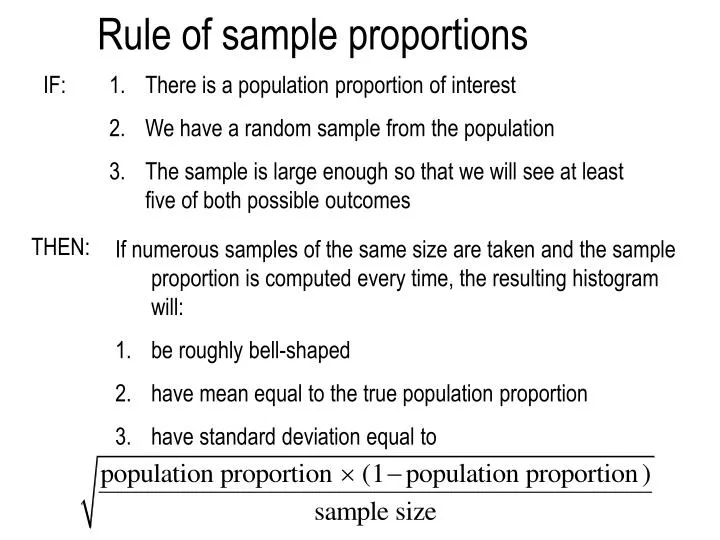
Rule of sample proportions. IF:. There is a population proportion of interest We have a random sample from the population The sample is large enough so that we will see at least five of both possible outcomes. THEN:.

E N D
Rule of sample proportions IF: • There is a population proportion of interest • We have a random sample from the population • The sample is large enough so that we will see at least five of both possible outcomes THEN: • If numerous samples of the same size are taken and the sample proportion is computed every time, the resulting histogram will: • be roughly bell-shaped • have mean equal to the true population proportion • have standard deviation equal to
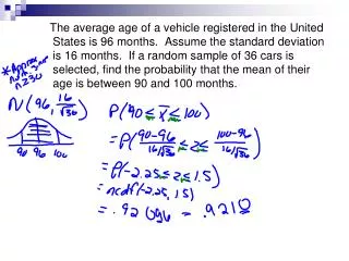
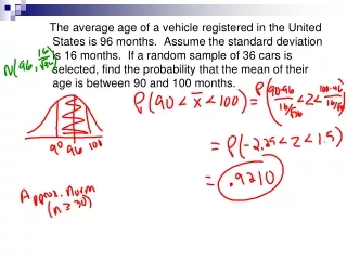
Sample means: measurement variables Suppose we want to estimate the mean weight at PSU Data from stat 100 survey, spring 2004. Sample size 237. Mean value is 152.5 pounds. Standard deviation is about (240 – 100)/4 = 35
What is the uncertainty in the mean? We need a margin of error for the mean. Suppose we take another sample of 237. What will the mean be? Will it be 152.5 again? Probably not. Consider what would happen if we took 1000 samples, each of size 237, and computed 1000 means.
Hypothetical result, using a “population” that resembles our sample: Extremely interesting: The histogram of means is bell-shaped, even though the original population was skewed! Standard deviation is about (157 – 148)/4 = 9/4 = 2.25
Formula for estimating the standard deviation of the sample mean (don’t need histogram) Just like in the case of proportions, we would like to have a simple formula to find the standard deviation of the mean without having to resample a lot of times. Suppose we have the standard deviation of the original sample. Then the standard deviation of the sample mean is:
So in our example of weights: The standard deviation of the sample is about 35. Hence by our formula: Standard deviation of the mean is 35 divided by the square root of 237: 35/15.4 = 2.3 (Recall we estimated it to be 2.25) So the margin of error of the sample mean is 2x2.3 = 4.6 Report 152.5 ± 4.6 (or 147.9 to 157.1)
Example: SAT math scores Suppose nationally we know that the SAT math test has a mean of 100 points and a standard deviation of 100 points. Draw by hand a picture of what you expect the distribution of sample means based on samples of size 100 to look like. Sample means have a normal distribution mean 500 standard deviation 100/10 = 10 So draw a bell shaped curve, centered at 500, with 95% of the bell between 500 – 20 = 480 and 500 + 20 = 520
A sample of 100 SAT math scores with a mean of 540 would be very unusual. A sample of 100 with a mean of 510 would not be unusual.
Rule of sample means IF: • The population of measurements of interest is bell-shaped, OR • A large sample (at least 30) is taken. THEN: • If numerous samples of the same size are taken and the sample mean is computed every time, the resulting histogram will: • be roughly bell-shaped • have mean equal to the true population mean • have standard deviation estimated by
Back to proportions:Suppose the true proportion is known When we know the true population proportion, then we can anticipate where a sample proportion will fall (give an interval of values). It is known that about 12% of the population is left-handed. Take a sample of size 200. We need the standard deviation of the sample proportion:
We want a normal curve centered at .12 with standard deviation .023. So 95% of the bell should be spread between .12 – 2(.023) = .12 − .046 = .074 .12 + 2(.023) = .12 + .046 = .166
95% of the time, we expect a sample of size 200 to produce a sample proportion between .074 and .166. 5% of the time, we expect the sample proportion to be outside this range.
True proportion known (cont’d) If you play 100 games of craps, where will the proportion of games you win lie 95% of the time? True proportion (mean of sample proportions): .493 Standard deviation of sample proportions: Answer: Between .493−2(.050) and .493+2(.050), or between .393 and .593.
True proportion unknown Next, suppose we do not know the true population proportion value. This is far more common in reality! How can we use information from the sample to estimate the true population proportion? Suppose we have a sample of 200 students in STAT 100 and find that 28 of them are left handed. Our sample proportion is: .14
We can now estimate the standard deviation of the sample proportion based on a sample of size 200: Hence, 2 standard deviations = 2(.025) = .05
Note the green curve, which is the truth. Of course, ordinarily we don’t know where it lies, but at least we know its standard deviation. Thus, we can build a confidence interval around our 14% estimate (in red). If we take another sample, the red line will move but the green curve will not!
If we repeat the sampling over and over, 95% of our confidence intervals will contain the true proportion of 0.12. This is why we use the term “95% confidence interval”.
Definition of “95% confidence interval for the true population proportion”: • An interval of values computed from the sample that is almost certain (95% certain in this case) to cover the true but unknown population proportion. • The plan: • Take a sample • Compute the sample proportion • Compute the estimate of the standard deviation of the sample proportion: • 95% confidence interval for the true population proportion: sample proportion ± 2(SD)