Download
1 / 61
610 likes | 611 Views
This guideline emphasizes the importance of starting with a simple model and gradually adding complexity based on the available hydrogeology data. It also highlights the tradeoff between model fit and prediction accuracy and the need to incorporate diverse observation data.

E N D
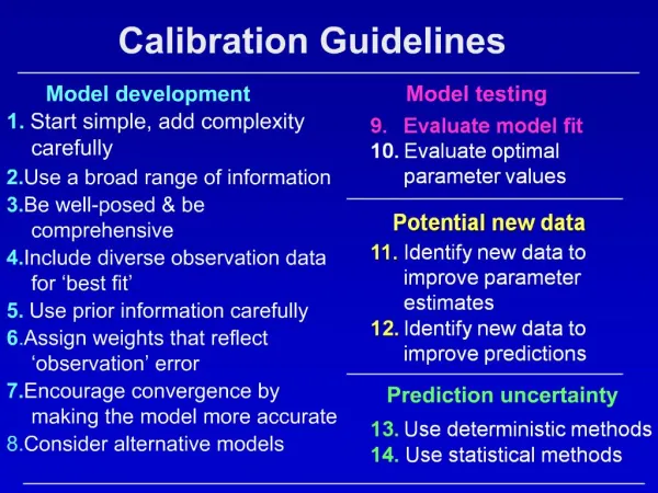
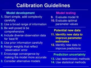
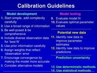
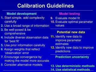
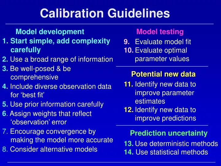
Calibration Guidelines Model development Model testing 9.Evaluate model fit 10.Evaluate optimal parameter values 11. Identify new data to improve parameter estimates 12. Identify new data to improve predictions 13.Use deterministic methods 14.Use statistical methods 1.Start simple, add complexity carefully 2. Use a broad range of information 3. Be well-posed & be comprehensive 4. Include diverse observation data for ‘best fit’ 5.Use prior information carefully 6. Assign weights that reflect ‘observation’ error 7. Encourage convergence by making the model more accurate 8. Consider alternative models Potential new data Prediction uncertainty
Model DevelopmentGuideline 1: Apply principle of parsimony(start simple, add complexity carefully) Start simple. Add complexity as warranted by the hydrogeology, the inability of the model to reproduce observations, the predictions, and possibly other things. But my system is so complicated!! DATA ARE LIMITED. SIMULATING COMPLEXITY NOT SUPPORTED BY THE DATA CAN BE USELESS AND MISLEADING.
Model complexity accuracy • Neither a million grid nodes nor hundreds of parameters guarantee a model capable of accurate predictions. • Here, we see that a model that fits all the data perfectly can be produced by adding many parameters, but the resulting model has poor predictive capacity. It is fitting observation error, not system processes. • We don’t know the ‘best’ level of complexity. We do know that we don’t want to start matching observation error. Observation error is evaluated when determining weights (Guideline 6).
model fit prediction error Model complexity accuracy Model simplicity accuracy • General situation: Tradeoff between model fit and prediction accuracy with respect to the number of parameters
Can 20% of the system detail explain 90% of the dynamics? • The principle of parsimony calls for keeping the model as simple as possible while still accounting for the main system processes and characteristics evident in the observations, and while respecting other system information. • Begin calibration by estimating very few parameters that together represent most of the features of interest. • The regression methods provide tools for more rigorously evaluating the relation between the model and the data, compared to trial and error methods. • It is expected (but not guaranteed) that this more rigorous evaluation produces more accurate models.
Flow through Highly Heterogeneous Fractured Rock at Mirror Lake, NH Tiedeman, et al., 1998
20% of the system detail does explain 90% of the dynamics! MODFLOW Model with only 2 horizontal hydraulic conductivity parameters Conceptual Cross Section Through Well Field Fracture zoneswith high T Fracture zones with high T Fractures with low T
Apply principle of parsimony to allaspects of model development • Start by simulating only the major processes • Use a mathematical model only as complex as is warranted. • When adding complexity, test: • Whether observations support the additional complexity • Whether the additional complexity affects the predictions This can require substantial restraint!!!
Advantages of starting simple and building complexity as warranted • Transparency: Easier to understand the simulated processes, parameter definition, parameter values, and their consequences. Can test whether more complexity matters. • Refutability: Easier to detect model error. • Helps maintain big picture view consistent with available data. • Often consistent with detail needed for accurate prediction. • Can build prediction scenarios with detailed features to test the effect f those features. • Shorter execution times
Computer execution time for inverse models can be approximated using the time for forward models and the number of parameters estimated (NP) as: Tinverse= 2(NP)Tforward(1+NP) (1+NP) is the number of solutions per parameter-estimation iteration 2(NP) is an average number of parameter estimation iterations To maintain overnight simulations, try for Tforward< about 30 minutes Tricks: Buffer sharp K contrasts where possible Consider linear versions of the problem as much as possible (for gw problems: replace the water table with assigned thickness unless the saturated thickness varies alot over time; replace nonlinear boundary conditions such as EVT and RIV Packages of MODFLOW with GHB Package during part of calibration) Parallel runs Issues of computer execution time
Calibration Guidelines Model development Model testing 9.Evaluate model fit 10.Evaluate optimal parameter values 11. Identify new data to improve parameter estimates 12. Identify new data to improve predictions 13.Use deterministic methods 14.Use statistical methods 1.Start simple, add complexity carefully 2.Use a broad range of information 3. Be well-posed & be comprehensive 4. Include diverse observation data for ‘best fit’ 5.Use prior information carefully 6. Assign weights that reflect ‘observation’ error 7. Encourage convergence by making the model more accurate 8. Consider alternative models Potential new data Prediction uncertainty
Model DevelopmentGuideline 2:Use a broad range of information (soft data)to constrain the problem • Soft data is that which cannot be directly included as observations in the regression • Challenge: to incorporate soft data into model so that it (1) characterizes the supportable variability of hydrogeologic properties, and (2) can be represented by a manageable number of parameters. • For example, in ground-water model calibration, use hydrology and hydrogeology to identify likely spatial and temporal structure in areal recharge and hydraulic conductivity, and use this structure to limit the number of parameters needed to represent the system. Do not add features to the model to attain model fit if they contradict other information about the system!!
Example: Parameterization for simulation of ground-water flow in fractured dolomite(Yager, USGS Water Supply Paper 2487, 1997) How to parameterize hydraulic conductivity in this complex system? Yager took advantage of data showing that the regional fractures that dominate flow are along bedding planes.
Example: Parameterization for simulation of ground-water flow in fractured dolomite • Transmissivity estimated from aquifer tests is roughly proportional to the number of fractures intersecting the pumped well. • Thus, assume all major fractures have equal T, and calculate T for each model layer from the number of fractures in the layer. • The heterogeneous T field can then be characterized by a single model parameter and multiplication arrays.
Data management, analysis, and visualization Data management, analysis, and visualization problems can be daunting. It is difficult to allocate project time between these efforts and modeling in an effective manner, because: • There are many kinds of data (point well data, 2D and 3D geophysics, cross sections, geologic maps, etc) and the subsurface is often very complex. Capabilities for integrating these data exist, but can be cumbersome. • The hardware and software change often. Thus far, products have been useful, but not dependable or comprehensive. • Low end: Rockworks ~US$2000. High end: Earthvision ~US$100,000 +US$20,000/yr GUI’s provide some capabilities
Calibration Guidelines Model development Model testing 9.Evaluate model fit 10.Evaluate optimal parameter values 11. Identify new data to improve parameter estimates 12. Identify new data to improve predictions 13.Use deterministic methods 14.Use statistical methods 1.Start simple, add complexity carefully 2. Use a broad range of information 3.Be well-posed & be comprehensive 4. Include diverse observation data for ‘best fit’ 5.Use prior information carefully 6. Assign weights that reflect ‘observation’ error 7. Encourage convergence by making the model more accurate 8. Consider alternative models Potential new data Prediction uncertainty
Model DevelopmentGuideline 3: Be Well-Posed & Be Comprehensive Well posed: Don’t spread observation data too thinlyFor a well-posed problem, estimated parameters are supported by the calibration observations, and the regression converges to optimal values. In earth systems, observations are usually sparse, so being well-posed often leads to models with few parameters. Comprehensive: Include many system aspects.Characterize as many system attributes as possible using defined model parameters. Leads to many parameters. Is achieving Guideline 3 possible? Challenge: Bridge the gap. Develop a useful model that has complexity the observation data can support and the predictions need.
Be Well-Posed and Be Comprehensive • Often harder to bewell posed than to be comprehensive. • Easy to add lots of complexity to a model. • Harder to limit complexity to what is supported by the observations and most important to predictions. • Keeping the model well-posed can be facilitated by: • Scaled sensitivities, parameter correlation coefficients, leverage statistics • Independent of model fit. Can use before model is calibrated • Cook’s D, DFBeta’s (influence statistics) • Advantage -- integrate sensitivities and parameter correlations. • Caution -- dependent on model fit. Use cautiously with uncalibrated model.
Dimensionless Scaled Sensitivities: Support of each observation for each parameter(example from Death Valley) • Estimation of parameter K4 seems to be dominated by 4 observations: 3 heads and 1 flow. • Scaled sensitivities neglect parameter correlation, so some observations may be more important than indicated. In ground-water problems, flows are very important for reducing correlations. Heads: obs # 1-501 Flows: obs # 502-517 3 dominant head obs 1 dominant flow obs
Composite Scaled Sensitivities: Support of whole observation set for each parameter • CSS for initial Death Valley model with only 9 parameters. • Graph clearly reveals relative support the observations as a whole provide towards estimating each parameter. • Observations provide much information about RCH and 2 or 3 of the K parameters; little information about ANIV or ETM Supportable model complexity The observations provide enough information to add complexity to the K and RCH parameterization
Composite Scaled Sensitivities: Support of whole observation set for each parameter Supportable model complexity Good way to show the observation support as the number of defined parameters becomes large. This graph is from the final Death Valley model. • Black bars: parameters estimated by regression. • Grey bars: not estimated by regression because of parameter correlation, insensitivity, or other reasons.
Parameter correlations: DVRFS model • pcc >0.95 for 4 parameter pairs in the three-layer DVRFS model with: • all 23 parameters active • no prior information • 501 head observations • 16 flow observations. • With head data alone, all parameters except vertical anisotropy are perfectly correlated -- Multiply all by any positive number, get identical head distribution. By Darcy’s Law. • The flow observations reduce the correlation to what is shown above.
Influence Statistics • Like DSS, they help indicate if parameter estimates are largely affected by just a few observations • Like DSS, they depend on the type, location, and time of the observation • Unlike DSS, they depend on model fit to the observed value. • Unlike DSS, they include the effect of pcc (parameter correlation coefficient) (Leverage does this, too) • Cook’s D: a measure of how a set of parameter estimates would change with omission of an observation, relative to how well the parameters are estimated given the entire set of observations.
Cook’s D – Which observations are most important to estimating all the parameters?(3-layer Death Valley example) Accounts for sensitivities, parameter correlations, and model fit • Estimation dominated by ~10% of the observations • 5 obs very important: 3 heads, 2 flows. • Importance of flows is better reflected by Cook’s D than scaled sensitivities. In gw problems, flows often resolve extreme correlation. Need flows to uniquely estimate parameter values. • Although dependent on model fit, relative valuesof Cook’s D can be useful for uncalibrated models. flow obs (502-517)
Sensitivity Analysis for 2 parameters • CSS • DSS • Leverage • Cook’s D • DFBETAS Conclusion: flow qleft has a small sensitivity but is critical to uncoupling otherwise completely correlated parameters.
Which statistics address which relations?? Observations – Parameters - Predictions dss pss css ppr pcc leverage Parameter cv AIC BIC DFBETAS Cook’s D opr Observations ---------------- Predictions
Problems with Sensitivity Analysis Methods • Nonlinearity of simulated values with respect to the parameters • Inaccurate sensitivities
Nonlinearity Nonlinearity: sensitivities differ for different parameter values. • Scaled sensitivities change for different parameter values because (1) the sensitivities are different and (2) the scaling. [dss= (y/b)bw1/2] • Consider decisions based on scaled sensitivities to be preliminary. Test by trying to estimate parameters. If conclusions drawn from scaled sensitivities about what parameters are important and can be estimated change dramatically for different parameter values, the problem may be too nonlinear for this kind of sensitivity analysis and regression to be useful. • Parameter correlation coefficients commonly differ for different parameter values. • Extreme correlation is indicated if pcc=1.0 for all parameter values; regression can look okay – but beware! (see example in Hill and Tiedeman, 2003) (pcc) From Poeter and Hill, 1997. See book p. 58
Inaccurate sensitivities How accurate are the sensitivities? • Most accurate: sensitivity-equation method. MODFLOW-2000. [Generally 5-7 digits] • Less accurate: Perturbation methods. UCODE_2005 or PEST. [Often only 2-3 digits] Both programs can use model-produced sensitivities if available. When does it NOT matter? • Scaled sensitivities, regression often do not require accurate sensitivities. Regression convergence improves with more accurate sensitivities for problems on the edge. [Mehl and Hill, 2002] When does it matter? • Parameter correlation coefficients. [Hill and Østerby, 2003] • Values of 1.00 and –1.00 reliably indicate parameter correlation; smaller absolute values do not guarantee lack of correlation unless the sensitivities are known to be sufficiently accurate. • Parameter correlation coefficients have more problems as sensitivity accuracy declines for all parameters, but it is most severe for pairs of parameters for which one parameter or both parameters have small composite scaled sensitivity.
Calibration Guidelines Model development Model testing 9.Evaluate model fit 10.Evaluate optimal parameter values 11. Identify new data to improve parameter estimates 12. Identify new data to improve predictions 13.Use deterministic methods 14.Use statistical methods 1.Start simple, add complexity carefully 2. Use a broad range of information 3. Be well-posed & be comprehensive 4.Include diverse observation data for ‘best fit’ 5.Use prior information carefully 6. Assign weights that reflect ‘observation’ error 7. Encourage convergence by making the model more accurate 8. Consider alternative models Potential new data Prediction uncertainty
Model Development Guideline 4:Include many kinds of data as observations (hard data) in the regression • Adding different kinds of data generally provides more information about the properties of the simulated system. • In ground-water flow model calibration • Flow data are important. With only head data, if all major K and Recharge parameters are being estimated, extreme values of parameter correlation coefficients will likely occur (Darcy’s Law). • Advective transport (or concentration first-moment data) can provide valuable information about the rate and direction of ground-water flow. • In ground-water transport model calibration • Advective transport (or concentration first-moment data) important because they are more stable numerically and the misfit increases monotonically as the fit to observations becomes worse. (Barth and Hill, 2005a,b, Journal of Contaminant Hydrology)
Here, model fit does not change with changes in the parameter values unless overlap occurs From Barth and Hill (2005a). Book p. 224
Contoured or kriged data values as ‘observations’?(book p. 284) • Has the advantage of creating additional ‘observations’ for the regression. • However, a significant disadvantage is that the interpolated values are not necessarily consistent with processes governing the true system, e.g. the physics of ground-water flow for the true system. For example, interpolated values could be unrealistically smooth across abrupt hydrogeologic boundaries in the true subsurface. • This can cause estimated parameter values to representative of the true system poorly. Proceed with Caution !!!!
Calibration Guidelines Model development Model testing 9.Evaluate model fit 10.Evaluate optimal parameter values 11. Identify new data to improve parameter estimates 12. Identify new data to improve predictions 13.Use deterministic methods 14.Use statistical methods 1.Start simple, add complexity carefully 2. Use a broad range of information 3. Be well-posed & be comprehensive 4. Include diverse observation data for ‘best fit’ 5.Use prior information carefully 6. Assign weights that reflect ‘observation’ error 7. Encourage convergence by making the model more accurate 8. Consider alternative models Potential new data Prediction uncertainty
nh 2 å = w - S ( b ) ( h h ' ( b )) i i i = i 1 Model DevelopmentGuideline 5: Use prior information carefully • Prior information allows some types of soft data to be included in objective function (e.g. T from aquifer test) • Prior information penalizes estimated parameter values that are far from ‘expected’ values through an additional term in the objective function. • What are the ‘expected’ values? +… HEADS FLOWSPRIOR
Hydrologic and hydrogeologic data: less accurate Relate to model inputs Dependent variable observations: more accurate Relate to model outputs - calibration Ground-Water Modeling Ground-Water Model -- Parameters Predictions Prediction uncertainty Societal decisions
Suggestions • Begin with no prior information, to determine the information content of the observations. • Insensitive parameters (parameters with small css): • Can include in regression using prior information to maintain a well-posed problem • Or during calibration exclude them to reduce execution time. Include them when calculating prediction uncertainty and associated measures (Guidelines 12 – 14). • Sensitive parameters: • Do not use prior information to make unrealistic optimized parameter values realistic. • Figure out why model + calibration data together cause regression to converge to unrealistic values (see Guideline 9).
Highly parameterized models • # parameters > # observations • Methods • Pilot points (de Marsily, RamaRao, LaVenue) • Pilot points with smoothing (Tikhonov) • Pilot points with regularization (Alcolea, Doherty) • Sequential self calibration (Gomez-Hernandez, Hendricks Franssen) • Representer (Valstar) • Moment mehod (Guadagnini, Neuman) • Most common current usage: PEST regularization capability, by John Doherty
Why highly parameterize? • Can easily get close fits to observations • Intuitive appeal to resulting distributions • We know the real field varies • Highly parameterized methods can be used to develop models with variable distributions • Mostly used to represent K; can use if for other aspects of the system
Why not highly parameterize? • Are the variations produced by highly parameterized fields real? • Perhaps NO if they are produced because of • Data error (erroneous constraint) • Lack of data (no constraint) • Instability • How can we know? • Here, consider synthetic problem. • Start with no observation error • Add error to observations
(From Hill and Tiedeman, 2006, Wiley) 11 Observations: 10 heads (*), 1 flow (to river) 6 Parameters: HK_1 HK_2 (multiplier) RCH_1, RCH_2 K_RB (prior) VK_CB (prior) Steady state . . . . . . .. . . . . . . . . . . . . . . . . . . . . . . . . . . . . * * * Top layer really homogeneous. Consider using 36 pilot points to represent it. * * * * * * * Model Layer 1 Model Layer 2
Initial run with no data error Here, use the constrained minimization regularization capability of PEST Variogram inputs: Nugget=0.0 a=3x10⁷ Variance=0.1 Interpolation inputs: Search radius=36,000 Max points=36 • Consistent with the constant value that actually occurs. Equals fit achieved with a single HK_1 parameter given a correct model and observations with no error Fit Criterion phi=1x10⁻⁵
Introducing variability • The variogram and interpolation input reflects a much better understanding of the true distribution than would • normally be the case. To create a more realistic • situation, use β, the regularization weight factor S(b)= (y-yobs)T w(y-yobs) + β(Δp-0)Tw (Δp-0) To the extent that β can be small, variability is allowed in the K distribution. Increased s2lnK
No data error. Correct model. Perform regression starting from values other than the true values Percent error for each parameter calculated as 100|(btrue-best)/btrue| For HK_1, best= exp(lnK) lnK=mean of the ln K’s of the 36 pilot points Also report s2lnK If β is restricted to be close to 1.0, the estimates are close to the true and s2lnK is small, as expected. What happens if β can be small?
No data error. Correct model. Perform regression starting from values other than the true values Percent error for each parameter calculated as 100|(btrue-best)/btrue| For HK_1, best= exp(lnK) lnK=mean of the ln K’s of the 36 pilot points s2ln(k)= 0.1 β=
No data error. Correct model. Perform regression starting from another set of values Same good fit to obs
No data error. Correct model. Parameter estimates depend on starting parameter values • Disturbing. • Means that in the following results as β becomes small discrepancies may not be caused by observation error.
Data error. Correct model. • Parameter error • Distribution of K in layer 1
Data error. Correct model. Parameter error s2 ln(k)= 1.2 Not possible to determine for which phi values will be accurate. Small parameter error Accurate predictions? Depends on effect of the variability.