Download
1 / 25
250 likes | 399 Views
C&O 355 Mathematical Programming Fall 2010 Lecture 2. N. Harvey. TexPoint fonts used in EMF. Read the TexPoint manual before you delete this box .: A A A A A A A A A A. Outline. LP definition & some equivalent forms Example in 2D Theorem: LPs have 3 possible outcomes Examples

E N D
C&O 355Mathematical ProgrammingFall 2010Lecture 2 N. Harvey TexPoint fonts used in EMF. Read the TexPoint manual before you delete this box.: AAAAAAAAAA
Outline • LP definition & some equivalent forms • Example in 2D • Theorem: LPs have 3 possible outcomes • Examples • Linear regression, bipartite matching, indep set • Solutions at corner points • Duality and certificates
Linear Program • General definition • Parameters: c, a1,…,am2Rn, b1,…,bm2R • Variables: x2Rn • Terminology • Feasible point: any x satisfying constraints • Optimal point: any feasible x that minimizes obj. func • Optimal value: value of obj. func for any optimal point Objective function Constraints
Linear Program • General definition • Parameters: c, a1,…,am2Rn, b1,…,bm2R • Variables: x2Rn • Matrix form • Parameters: c2Rn, A2Rm£n, b2Rm • Variables: x2Rn
Simple LP Manipulations • “max” instead of “min” max cT x ´ min –cT x • “¸” instead of “·” aTx¸ b , -aTx· -b • “=” instead of “·” aTx=b , aTx· b and aTx¸ b • Note: “<“ and “>” are not allowed in constraintsBecause we want the feasible region to be closed, in the topological sense.
2D Example Objective Function Constraint x2 Optimal point x2 - x1· 1 (3,2) x1 + 6x2· 15 Feasible region Gradient ofObjective Function x2¸0 x1 (0,0) x1¸0 4x1 - x2· 10 Unique optimal solution exists
2D Example Objective Function Constraint x2 Optimal points x2 - x1· 1 x1 + 6x2· 15 Feasible region Gradient ofObjective Function x2¸0 x1 (0,0) x1¸0 4x1 - x2· 10 Optimal solutions exist: Infinitely many!
2D Example Constraint x2 x2 - x1¸ 1 x1 + 6x2· 15 Feasible regionis empty Gradient ofObjective Function x2¸0 x1 (0,0) x1¸0 4x1 - x2¸ 10 Infeasible No feasible solutions(so certainly no optimal solutions either)
2D Example Constraint x2 x2 - x1· 1 Gradient ofObjective Function x2¸0 x1 (0,0) x1¸0 Feasible region Unbounded Feasible solutions, but no optimal solution (Informally, “optimal value = 1”)
2D Example Constraint x2 x2 - x1· 1 Optimal point (0,1) Gradient ofObjective Function x2¸0 x1 (0,0) Feasible region x1¸0 Important Point: This LP is NOTunbounded. The feasible region is unbounded,but optimal value is 1
“Fundamental Theorem” of LP • Theorem: For any LP, the outcome is either: • Optimal solution (unique or infinitely many) • Infeasible • Unbounded(optimal value is 1 for maximization problem,or -1 for minimization problem) • Proof: Later in the course!
Example: Linear regression • Given data (x1, y1), …, (xn, yn) in R2 • Find a line y = ax + b that fits the points Usual setup Our setup Easy: differentiate, set to zero Not differentiable! • Absolute value trick: ´ • Our setup can be written as an LP
Example: Bipartite Matching • Given bipartite graph G=(V, E) • Find a maximum size matching • A set Mµ E s.t. every vertex has at most one incident edge in M
Example: Bipartite Matching • Given bipartite graph G=(V, E) • Find a maximum size matching • A set Mµ E s.t. every vertex has at most one incident edge in M The blue edges are a matching M
Example: Bipartite Matching • Given bipartite graph G=(V, E) • Find a maximum size matching • A set Mµ E s.t. every vertex has at most one incident edge in M • The natural integer program (IP) • Solving IPs is very hard. Try an LP instead. (LP) • Theorem: (IP) and (LP) have the same solution! • Proof: Later in the course! • Corollary: Bipartite matching can be solved by LP algorithms.
Example: Independent Set(a.k.a., Stable Set, or Coclique, or Anti-Clique) • Given graph G=(V, E) • Find a maximum size independent set • A set UµV s.t. {u,v} E for every distinct u,v2U
Example: Independent Set • Given graph G=(V, E) (assume no isolated vertices) • Find a maximum size independent set • A set UµV s.t. {u,v} E for every distinct u,v2 U • Write an integer program (IP) • Solving IPs is very hard. Try an LP instead. (LP) • Unfortunately (IP) and (LP) are extremely different. • Fact: For any n, there are graphs with |V|=n such thatOPTLP / OPTIP¸ n/2.
Example: Independent Set • Given graph G=(V, E) • Find a maximum size independent set • A set UµV s.t. {u,v} E for every distinct u,v2 U • Write an integer program (IP) • Solving IPs is very hard. Try an LP instead. (LP) • In fact, there is a (difficult) theorem in Complexity Theory which says (roughly) that Maximum Independent Set cannot be efficiently solved any better than (LP) does.
Where are optimal solutions? x2 x2 - x1· 1 x1 + 6x2· 15 x1 4x1 - x2· 10
Where are optimal solutions? x2 x2 - x1· 1 x1 + 6x2· 15 x1 4x1 - x2· 10
Where are optimal solutions? x2 x2 - x1· 1 x1 + 6x2· 15 x1 4x1 - x2· 10 Lemma: For any LP, a “corner point” is an optimal solution. (Assuming an optimal solution exists and some corner point exists). Proof: Later in the course!
Duality George Dantzig1914-2005 “Another key visit took place in October 1947 at the Institute for Advanced Study (IAS) where Dantzig met with John von Neumann. Dantzig recalls, “I began by explaining the formulation of the linear programming model… I described it to him as I would to an ordinary mortal. ‘Get to the point,’ he snapped. In less than a minute, I slapped the geometric and algebraic versions of my problem on the blackboard. He stood up and said, ‘Oh that.’” Just a few years earlier von Neumann had co-authored his landmark monograph on game theory. Dantzig goes on, “for the next hour and a half he proceeded to give me a lecture on the mathematical theory of linear programs.” Dantzig credited von Neumann with edifying him on Farkas’ lemma and the duality theorem (of linear programming).” from http://www.ams.org/notices/200703/fea-cottle.pdf
Duality: Proving optimality • Question: What is optimal point in direction c = (-7,14)? • Solution: Optimal point is x=(9/7,16/7), optimal value is 23. • How can I be sure? • Every feasible point satisfies x1+6x2· 15 • Every feasible point satisfies -x1+x2· 1 • Every feasible point satisfies their sum: -7x1+14x2· 23 ) -8x1+8x2· 8 This is the objective function! x2 (9/7,16/7) -x1+x2· 1 x1 + 6x2· 15 x1 4x1 - x2· 10
Duality: Proving optimality • Question: What is optimal point in direction c = (-7,14)? • Solution: Optimal point is x=(9/7,16/7), optimal value is 23. • How can I be sure? • Every feasible point satisfies x1+6x2· 15 • Every feasible point satisfies -x1+x2· 1 ) -8x1+8x2· 8 • Every feasible point satisfies their sum: -7x1+14x2·23 This is the objective function! • Certificates • To convince you that optimal value is ¸ k, I can find x such that cT x ¸ k. • To convince you that optimal value is ·k, I can find a linear combination of the constraints which proves that cT x · k. • Theorem: Such certificates always exists. • Proof: Later in the course!