Download
1 / 47
470 likes | 480 Views
Converting POLYMATH Solutions to MATLAB Files Introduction WHY MATLAB FOR NUMERICAL PROBLEM SOLVING? LARGE SCALE, COMPLEX PROBLEMS MAY REQUIRE PROGRAMMING BY EITHER MATLAB OR A PROGRAMMING LANGUAGE (C, PASCAL OR FORTRAN). WHY USE A POLYMATH PREPROCESSOR ?

E N D
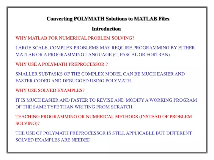
Converting POLYMATH Solutions to MATLAB Files Introduction WHY MATLAB FOR NUMERICAL PROBLEM SOLVING? LARGE SCALE, COMPLEX PROBLEMS MAY REQUIRE PROGRAMMING BY EITHER MATLAB OR A PROGRAMMING LANGUAGE (C, PASCAL OR FORTRAN). WHY USE A POLYMATH PREPROCESSOR ? SMALLER SUBTASKS OF THE COMPLEX MODEL CAN BE MUCH EASIER AND FASTER CODED AND DEBUGGED USING POLYMATH. WHY USE SOLVED EXAMPLES? IT IS MUCH EASIER AND FASTER TO REVISE AND MODIFY A WORKING PROGRAM OF THE SAME TYPE THAN WRITING FROM SCRATCH. TEACHING PROGRAMMING OR NUMERICAL METHODS (INSTEAD OF PROBLEM SOLVING)? THE USE OF POLYMATH PREPROCESSOR IS STILL APPLICABLE BUT DIFFERENT SOLVED EXAMPLES ARE NEEDED.
1 ONE NONLINEAR ALGEBRAIC EQUATION - FZERO – SLIDES 3-9 2 SYSTEMS OF NONLINEAR ALGEBRAIC EQUATIONS – FSOLVE – SLIDES 10-14 3 ODE – INITIAL VALUE PROBLEMS – ODE45 – SLIDES 15-20 4 ODE – BOUNDARY VALUE PROBLEMS – FZERO+ODE45 – SLIDES 21-26 5 DAE – INITIAL VALUE PROBLEMS – ODE45+FZERO – SLIDES 27-31 6 PARTIAL DIFFERENTIAL EQS – METHOD OF LINES+ODE45 – SLIDE 32 7 MULTIPLE LINEAR REGRESSION – MLIN_REG – SLIDES 33-37 8 POLYNOMIAL REGRESSION – POLY_REG – SLIDES 38-42 9 MULTIPLE NONLINEAR REGRESSION – NLN_REG – SLIDES 43-47 CONVERTING POLYMATH SOLUTIONS TO MATLAB FILES TYPES OF PROBLEMS DISCUSSED
ONE NONLINEAR ALGEBRAIC EQUATION FUNCTIONS (1) CONVERSION OF MOST OF THE PROBLEM TYPES REQUIRES CONVERSION OF THE POLYMATH MODEL INTO A MATLAB FUNCTION TO PREPARE THE FUNCTIONS COPY THE IMPLICIT EQUATION AND THE ORDERED EXPLICIT EQUATIONS FROM THE POLYMATH SOLUTION REPORT: (demonstrated in reference to Demo 2). Nonlinear equations [1] f(V) = (P+a/(V^2))*(V-b)-R*T = 0 Explicit equations [1] P = 56 [6] Pr = P/Pc [2] R = 0.08206 [7] a = 27*(R^2*Tc^2/Pc)/64 [3] T = 450 [8] b = R*Tc/(8*Pc) [4] Tc = 405.5 [9] Z = P*V/(R*T) [5] Pc = 111.3
%filename fun_d2 %Note: file name=function name function f=fun_d2(x) % Function definition added V=x(1); % Variable definition added P = 56; % Adding semi-colon to suppress printing R = 0.08206; T = 450; Tc = 405.5; Pc = 111.3; Pr = P/Pc; a = 27*(R^2*Tc^2/Pc)/64; b = R*Tc/(8*Pc); Z = P*V/(R*T); f = (P+a/(V^2))*(V-b)-R*T; % Function value definition modified ONE NONLINEAR ALGEBRAIC EQUATION - FUNCTIONS (2) Paste the equations into the MATLAB editor and remove the text and the equation numbers. Add the first line as the function definition and the second line as the definition of the unknown. Revise the nonlinear equation and put it as the last equation. Put a semi colon after each equation.
%file name demo_2 clear, clc, format short g xguess=0.5; disp(‘Demo 2. Variable values at the initial estimate'); dsp_d2(xguess); %display the variable values at the initial estimate xsolv = fzero('fun_d2',xguess); %Use fzero to solve the equation disp(‘Demo 2. Variable values at the solution'); dsp_d2(xsolv); %display the variable values at the solution ONE NONLINEAR ALGEBRAIC EQUATION – THE DRIVER PROGRAM Use the following driver program (m-file) to obtain the basic solution of a system containing one implicit nonlinear algebraic equation and several explicit equations. MATLAB function used: fzerowith the basic calling sequence: X = FZERO(FUN,X0), where X0 is a starting guess (a scalar value). The algorithm looks first for an interval containing a sign change for FUN and containing X0 then it uses a combination of bisection, secant and inverse quadratic interpolation. Type help fzero in the MATLAB command window for more information
ONE NONLINEAR ALGEBRAIC EQUATION RUNNING THE DEMO SOLUTIONS CREATE A NEW FOLDER (SAY session_16) TO STORE THE FILES “SET PATH” FROM THE MATLAB COMMAND WINDOW TO THIS FOLDER AND SAVE THE PATH OPEN THE Demos_Matlab.xls FILE AND SELECT THE Demo 2 WORKSHEET COPY THE demo_2 M-FILE, PASTE IT AS A NEW M-FILE IN THE MATLAB EDITOR’S WINDOW AND SAVE THE FILE IN THE session_16 FOLDER REPEAT THIS PROCESS FOR THE FILES fun_d2 AND dsp_d2 (NOTE THAT dsp_d2 IS VERY SIMILAR TO fun_d2 EXCEPT THAT IT DOES NOT HAVE AN OUTPUT VARIABLE AND THE SEMI-COLONS ARE REMOVED FROM THE ENDS OF THE COMMANDS) TYPE IN demo_2 IN THE MATLAB COMMAND WINDOW NOTE THAT THE demo_2 DRIVER PROGRAM SOLVES BOTH PARTS A AND B OF THE DEMO 2 PROBLEM AND PLOTS THE RESULTS
Demo 2. Variable values at the initial estimate Demo 2. Variable values at the solution V = 0.5 V = 0.57489 P = 56 P = 56 R = 0.08206 R = 0.08206 T = 450 T = 450 Tc = 405.5 Tc = 405.5 Pc = 111.3 Pc = 111.3 0.50314 Pr = 0.50314 Pr = a = a = 4.1969 4.1969 b = 0.037371 b = 0.03737 Z = 0.75825 Z = 0.87183 f = -3.2533 f = 0 Zero found in the interval: [0.42, 0.58]. One Nonlinear Algebraic Equation Functions, Results In the function: dsp_d2 only the function definition line is changed to: function dsp_d2(x)and the semi colons are removed from the ends of the equations. The results rearranged in two columns are:
%file name demo_2 clear, clc, format short g global Pr Z P Pr_set=[1 2 4 10 20]; xsolv=0.5; %initial estimate for the first V for j=1:5 Pr=Pr_set(j); xguess = xsolv; %use the previous solution as initial estimate xsolv=fzero(‘fun_d2’,xguess); %use fsolve to solve the equation/s V_set(j,1)=xsolv; P_set(j,1)=P; Z_set(j,1)=Z; end One Nonlinear Algebraic Equation Revising the Program for Parametric Runs (1) After the correct solution for one case has been obtained the driver program can be changed to solve the problem for different parameter values and to present the results in tabular and graphic forms. This particular example is solved for Pr = 1, 2, 4, 10 and 20. The results, including the pressure (P), reduced pressure (Pr), molar volume (V) and compressibility factor (Z) are presented in tabular form and Z is plotted versus Pr. The parameter Pr and the variables P and Z are defined as global variable in the driver program and in the function:
disp(' Compressibility Factor at 450 K for Ammonia'); Compressibility Factor at 450 K for Ammonia disp(' P (atm) Pr V(L/g-mol) Z') P(atm) Pr V(L/g-mol) Z Res=[P_set Pr_set V_set Z_set]; 111.3 1 0.23351 0.70381 disp (Res); 222.6 2 0.077268 0.46578 plot(Pr_set,Z_set,'-') 445.2 4 0.060654 0.73126 title(['Compressibility factor versus reduced pressure, ']); 1113 10 0.050875 1.5334 xlabel('Reduced pressure (Pr).'); 2226 20 0.046175 2.7835 ylabel('Compressibility factor (Z)'); One Nonlinear Algebraic Equation Revising the Program for Parametric Runs (2) This driver program prints the following tabular results:
%file name demo_5 clear, clc, format short g format compact xguess=[0 0 0]; % Row vector disp(‘Demo 5. Variable values at the initial estimate'); dsp_d5(xguess); options = optimset('Diagnostics',['off'],'TolFun',[1e-9],'TolX',[1e-9]); % Reduce to minimum warning messages issued by fsolve and % set convergence error tolerances xsolv=fsolve('fun_d5',xguess,options); %Use fsolve to solve the equation/s disp(‘Demo 5. Variable values at the solution'); dsp_d5(xsolv); Systems of Nonlinear Algebraic Equations Driver Program (1) To obtain a basic solution of a system containing several implicit nonlinear algebraic equations and several explicit equations use the following driver program (m-file):
Systems of Nonlinear Algebraic Equations Driver Program (2) This driver uses the MATLAB function fsolveto solve the system of nonlinear algebraic equations. The basic calling sequence: X=FSOLVE(FUN,X0, OPTIONS) starts at the row vector of initial estimates X0 and tries to solve the equations described in FUN. FUN is an M-file, which returns an evaluation of the equations for a particular value of X: F=FUN(X). The solution algorithms used by FSOLVE are based on nonlinear least- squares minimization. The default (large-scale) algorithm is the interior-reflective Newton method where every iteration involves the approximate solution of a large linear system using the method of preconditioned conjugate gradients. Optionally the Gauss-Newton method with line search or the Levenberg-Marquardt method with line search can be used. OPTIONS should be set to change default values of the FSOLVE parameters. The options that should often be changed include: Diagnostics, TolFun, TolX, MaxFunEvals and MaxIter. Complete list of the FSOLVE parameters and detailed description can be obtained by typing HELP OPTIMSET at the MATLAB command line.
Systems of Nonlinear Algebraic Equations Functions (1) To use the driver program shown above, the user has to provide two functions: fun_d5 (≡FUN) for calculating the function values and the function dsp_d5 to display the values of all the variables at the initial estimate and at the solution. The preparation of the two functions is demonstrated in reference to Demo 5. To prepare the functions copy the implicit equations and the ordered explicit equations from the POLYMATH solution report: Nonlinear equations [1] f(CD) = CC*CD-KC1*CA*CB = 0 [2] f(CX) = CX*CY-KC2*CB*CC = 0 [3] f(CZ) = CZ-KC3*CA*CX = 0 Explicit equations [1] KC1 = 1.06 [2] CY = CX+CZ [3] KC2 = 2.63 [4] KC3 = 5 [5] CA0 = 1.5 [6] CB0 = 1.5 [7] CC = CD-CY [8] CA = CA0-CD-CZ [9] CB = CB0-CD-CY
Systems of Nonlinear Algebraic Equations Functions (2) Paste the equations into the MATLAB editor and remove the text and the equation numbers. Add the first line as the function definition and insert directly after that the definition of the unknowns. Revise the nonlinear equations and put them as the last lines of the function. Put a semi colon after each equation. function f=fun_d5(x) % Function definition added %filename fun_d5 CX=x(2); % x is a row vector CD=x(1); % Variable definition added CZ=x(3); % Variable definition added CY = CX+CZ; KC1 = 1.06; KC2 = 2.63; KC3 = 5; CA0 = 1.5; CB0 = 1.5; CC = CD-CY; CB = CB0-CD-CY; CA = CA0-CD-CZ; f(1) = CC*CD-KC1*CA*CB; % Function value definition modified f(2) = CX*CY-KC2*CB*CC; % f is a row vector f(3) = CZ-KC3*CA*CX; % Function value definition modified
Problem D5. Variable values at the initial estimate Problem D5. Variable values at the solution CD= 0 CD = 0.70533 CX = 0 CX = 0.17779 CZ = 0 CZ = 0.37397 KC1 = 1.06 KC1 = 1.06 CY = 0 CY = 0.55176 KC2 = 2.63 KC2 = 2.63 KC3 = 5 KC3 = 5 CA0 = 1.5 CA0 = 1.5 CB0 = 1.5 CB0 = 1.5 CC = 0 CC = 0.15356 CA = 1.5 CA = 0.4207 CB = 1.5 CB = 0.24291 f1 = -2.385 f1 = -1.22E-05 f2 = 0 f2 = -7.04E-06 f3 = 0 f3 = -2.13E-06 Optimization terminated successfully: Systems of Nonlinear Algebraic Equations Functions, Results In the function: dsp_d5the function definition line is changed to: function dsp_d5(x), the semicolons are removed from the end of the equations and the function values are defined as scalars: f1, f2 and f3. Running the driver program yields the following results (some extra spaces were removed and the results were rearranged in two columns):
%file name demo_7 clear, clc, format short g tstart=0; %Initial value of the independent variable tfinal=200; %Final value of the independent variable y0=[20; 20; 20]; % Initial values of the dependent variables. A column vector disp(‘Demo 7. Variable values at the initial point'); dsp_d7(tstart,y0); [t,y]=ode45('dydt_d7',[tstart tfinal],y0); disp(Demo 7. Variable values at the final point'); [m,n]=size(y); % Find the address of the last point dsp_d7(tfinal,y(m,:)); plot(t,y(:,1),'+',t,y(:,2),'*',t,y(:,3),'o'); legend('T1','T2','T3'); title(' Heat Exchange in a Series of Tanks') xlabel('Time (min)'); ylabel('Temperature (deg. C)'); Ordinary Differential Equations – Initial Value Problems Driver Program (1)
Ordinary Differential Equations – Initial Value Problems Driver Program (2) This driver uses the MATLAB function ode45 to integrate the system of ODEs. The basic calling sequence: [T,Y] = ODE45('F',TSPAN,Y0) with TSPAN = [T0 TFINAL] integrates the system of differential equations y' = F(t,y) from time T0 to TFINAL with initial conditions Y0. 'F' is a string containing the name of an ODE file. Function F(T,Y) must return a column vector. The algorithm used is the variable step-size, explicit, 5th order Runge-Kutta (RK) method where the 4th order RK step is used for error estimation. If the system of ODEs is known to be stiff, or the RK method progresses very slowly the ODE15S function, which uses backward differential formulas (Gear’s method) is recommended. To use this driver program the user has to provide two functions: dydt_d7 (≡F) for calculating the derivative values at time = t, and the function dsp_d7 to display the values of all the variables at t = T0 and at t = TFINAL. The preparation of these two functions is demonstrated in reference to Demo 7.
Ordinary Differential Equations – Initial Value Problems Functions (1) To prepare the functions, copy the differential equations and the ordered explicit equations from the POLYMATH solution report: Paste the equations into the MATLAB editor. Add the first line as the function definition and insert directly after that the definition of the variables that are defined by differential equations. Put the explicit algebraic equations after the variable definition. Rewrite the differential equations in a column matrix form and put them as the last lines of the function. Differential equations as entered by the user [1] d(T1)/d(t) = (W*Cp*(T0-T1)+UA*(Tsteam-T1))/(M*Cp) [2] d(T2)/d(t) = (W*Cp*(T1-T2)+UA*(Tsteam-T2))/(M*Cp) [3] d(T3)/d(t) = (W*Cp*(T2-T3)+UA*(Tsteam-T3))/(M*Cp) Explicit equations as entered by the user [1] W = 100 [2] Cp = 2.0 [3] T0 = 20 [4] UA = 10. [5] Tsteam = 250 [6] M = 1000
%filename dydt_d7 function dydt=dydt_d7(t,y) %Function name added, y and dydt column vectors T1=y(1); %Variable definitions for T1,T2 and T3 are added T2=y(2); T3=y(3); W=100; Cp=2.0; T0=20; UA=10; Tsteam=250; M=1000; dydt=[(W*Cp*(T0-T1)+UA*(Tsteam-T1))/(M*Cp); %Differential equations modified (W*Cp*(T1-T2)+UA*(Tsteam-T2))/(M*Cp); (W*Cp*(T2-T3)+UA*(Tsteam-T3))/(M*Cp)]; Ordinary Differential Equations – Initial Value Problems Functions (2) In the function: dsp_d7the function definition line is changed to: function dsp_d7(t,y), the semicolons are removed and the derivative values are defined as scalars: dT1dt, dT2dt and dT3dt:
Demo7. Variable values at the initial point Demo7. Variable values at the final point T1 = 20 T1 = 30.952 T2 = 20 T2 = 41.383 T3 = 20 T3 = 51.317 W = 100 W = 100 Cp = 2 Cp = 2 T0 = 20 T0 = 20 UA = 10 UA = 10 Tsteam = 250 Tsteam = 250 M = 1000 M = 1000 dT1dt = 1.15 dT1dt = 1.37E-08 dT2dt = 1.15 dT2dt = 3.25E-08 dT3dt = 1.15 dT3dt = 6.66E-07 Ordinary Differential Equations – Initial Value Problems Tabular results Running the driver program yields the following results (some extra spaces were removed and the results were rearranged in two columns):
Ordinary Differential Equations – Initial Value Problems Graphic Results
%file name demo_8 clear, clc, format short g yi=-150; % Initial estimate for initial value of the second variable tstart=0; tfinal=0.001; y0=[0.2;yi]; % y is column vector, initial value for y(2) is sought disp(‘Demo 8. Variable values at the initial estimate'); dsp_d8(tstart,y0); yguess=yi; ysolv=fzero('fun_d8',yguess); %Use fzero to find initial value of y(2) y0=[0.2;ysolv]; % ysolv is the initial value of the second variable disp('Demo 8. Variable values at the initial point of the solution'); dsp_d8(tstart,y0); [t,y]=ode45('dydt_d8',[tstart tfinal],y0); disp(‘Demo 8. Variable values at the final point of the solution'); [m,n]=size(y); % Find the address of the last point dsp_d8(tfinal,y(m,:)); Ordinary Differential Equations – Boundary Value Problems Driver Program (1)
Ordinary Differential Equations – Boundary Value Problems Driver Program (2) In this particular example (Demo 8) the initial value for y(1) and the final value for y(2) are specified. This driver uses the MATLAB function ode45 in an inner loopto integrate the system of ODEs for an estimated value of y0(2). In the outer loop it uses the function fsolve to find y0(2) so thatat t = 0.001 y(2) = 0. Some more details concerning the functions fsolve and ode45 are provided in sections 1 and 3, respectively. To use this driver program the user has to provide three functions: dydt_d8 for calculating the derivative values at time = t, the function fun_d8 that calls dydt_d8 to calculate the value of y(2) at t = 0.001 and the function dsp_d8 to display the values of all the variables at t = T0 and at t = TFINAL. The preparation of these two functions is demonstrated in reference to Demo 8..
Ordinary Differential Equations – Boundary Value Problems Functions To prepare the function dydt_d8 copy the differential equations and the ordered explicit equations from the POLYMATH solution report: Paste the equations into the MATLAB editor and remove the text and the equation numbers. Add the first line as the function definition and insert directly after that the definition of the variables that are defined by differential equations. Put the explicit algebraic equations after the variable definition. Rewrite the differential equations in a column matrix form and put them as the last lines of the function. Put semi colons after each equation. Differential equations as entered by the user [1] d(CA)/d(z) = y [2] d(y)/d(z) = k*CA/DAB Explicit equations as entered by the user [1] k = 0.001 [2] DAB = 1.2E-9
%filename dydt_d8 %filename dsp_d8 function dydt=dydt_d8(t,y) %Function name added, y and dydt are column vectors function dsp_d8(t,y) CA=y(1); %Variable definition added CA=y(1) k=0.001; k=0.001 DAB=1.2e-9; DAB=1.2e-9 dydt=[y(2); k*CA/DAB]; %Differential equations modified dCAdz=y(2) dydz=k*CA/DAB Ordinary Differential Equations – Boundary Value Problems Functions (2) In the function: dsp_d8the semi colons are removed from the end of the equations and the derivative values are defined as scalars: dCAdz and dydz:
%filename fun_d8 function f=fun_d8(x) tstart=0; tfinal=0.001; y0=[0.2;x]; [t,y]=ode45('dydt_d8',[tstart tfinal],y0); [m,n]=size(y); f = y(m,2); % The final value of the second variable should be zero Ordinary Differential Equations – Boundary Value Problems Functions (3) The function fun_d8 has no equivalent in the POLYMATH file and it should be prepared so that it obtains the initial value y0(2) and returns the value of y(2) at t=0.001:
Demo 8. Variable values at the initial estimate CA = 0.2 k = 0.001 DAB = 1.20E-09 dCAdz = -150 dydz = 1.67E+05 Demo 8. Variable values at the initial point of the solution CA = 0.2 k = 0.001 DAB = 1.20E-09 dCAdz = -131.91 dydz = 1.67E+05 Demo 8. Variable values at the final point of the solution CA = 1.38E-01 k = 0.001 DAB = 1.20E-09 dCAdz = 3.02E-14 dydz = 1.15E+05 Ordinary Differential Equations – Boundary Value Problems Tabular results It can be seen that at the solution y0(2) = -131.91 (dCAdz) and at t=0.001 y(2) = 3.02E-14, very close to zero, indeed.
%file name demo_11 clear, clc, format short g tstart=0.4; tfinal=0.8; y0=[100]; disp(‘Demo 11 . Variable values at the initial point'); dsp_d11 (tstart,y0); [t,y]=ode45('dydt_d11',[tstart tfinal],y0); disp(‘Demo 11. Variable values at the final point'); [m,n]=size(y); dsp_d11(tfinal,y(m,:)); plot(t,y(:,1)); title(' Demo 11- Batch distillation of an ideal binary mixture ') xlabel('mole fraction of toluene'); ylabel('Amount of liquid'); Differential Algebraic Equations – Initial Value Problems Driver Program (1) To obtain a basic solution of a system containing one or more first order, ordinary differential equations, one or more implicit algebraic equations and several explicit equations the driver program used for ODE can be applied:
Differential equations as entered by the user Explicit equations as entered by the user [1] d(L)/d(x2) = L/(k2*x2-x2) [1] Kc = 0.5e6 [2] d(T)/d(x2) = Kc*err [2] k2 = 10^(6.95464-1344.8/(T+219.482))/(760*1.2) [3] x1 = 1-x2 [4] k1 = 10^(6.90565-1211.033/(T+220.79))/(760*1.2) [5] err = (1-k1*x1-k2*x2) Differential Algebraic Equations – Initial Value Problems Functions (1) This driver uses the MATLAB function ode45 to integrate the system of ODEs. To use this driver program the user has to provide two functions: dydt_d11 for calculating the derivative values at time = t, and the function dsp_d11 to display the values of all the variables at t = T0 and at t = TFINAL. The preparation of these two functions is demonstrated in reference to Demo 11. To prepare the function dydt_d11 copy the differential equations and the ordered explicit equations from the POLYMATH solution report:
Differential Algebraic Equations – Initial Value Problems Functions (2) The POLYMATH equations involve the use of the “controlled integration” method (Shacham et. al [2]) for solving the implicit algebraic equation. The same method can be used in the MATLAB solution. Here we use a different technique to show that this method yields the same results as the controlled integration method. Using this technique the equation: f(T) = 1- k1x1- k2x2 = 0 is solved at every integration step. The MATLAB function fzero is used to solve this nonlinear equation where the equation is defined as an “inline” function. The inline function definition enables to avoid the definition of an additional file. To convert the POLYMATH equation set into the function dydt_d11 copythe equations into the MATLAB editor and . Add the first line as the function definition and insert directly after that the definition of the variable: L = y(1). Put the explicit algebraic equations after the variable definition. Include a call to fzero to find the value of T, which satisfies the implicit algebraic equation. Rewrite the remaining single differential equation as an element in a column vector and put it as the last line of the function.
%filename dydt_d11 function dydt=dydt_d11(t,y) L=y(1); x2=t; T0=95; options=optimset('Display','off'); %Suppress printing some warning messages T=fzero(inline('1- 10^(6.90565-1211.033/(T+220.79))/(760*1.2)*(1-x2)- 10^(6.95464-1344.8/(T+219.482))/(760*1.2)*x2'),T0,options,x2); k2 = 10^(6.95464-1344.8/(T+219.482))/(760*1.2); k1 = 10^(6.90565-1211.033/(T+220.79))/(760*1.2); dydt=[L/(k2*x2-x2)]; Differential Algebraic Equations – Initial Value Problems Functions (3)
Demo 11 . Variable values at the initial point Demo 11. Variable values at the final point L = 100 L = 14.059 x2 = 0.4 x2 = 0.8 T0 = 95 T0 = 95 T = 95.585 T = 108.57 k2 = 0.53253 k2 = 0.78582 k1 = 1.31E+00 k1 = 1.8567 dLdz = -534.8 dLdz = -82.051 f = -1.69E-15 f = -1.11E-16 Differential Algebraic Equations – Initial Value Problems Solution An edited copy of the function dydt_d11, wherethe semi colons are removed from the end of the equations and the derivative value is defined as a scalar: dLdz, is used to display the results (function dsp_d11).Running the driver program yields the following results (some extra spaces were removed and the results were rearranged in two columns):
function dydt=dydt_d12(t,y) alpha = 2.e-5; T2=y(1); deltax = .10; T3=y(2); dydt=[ alpha/deltax^2*(T3-2*T2+T1); T4=y(3); alpha/deltax^2*(T4-2*T3+T2); alpha/deltax^2*(T5-2*T4+T3); T5=y(4); alpha/deltax^2*(T6-2*T5+T4); T6=y(5); T7=y(6); alpha/deltax^2*(T7-2*T6+T5); T8=y(7); alpha/deltax^2*(T8-2*T7+T6); alpha/deltax^2*(T9-2*T8+T7); T9=y(8); T10=y(9); alpha/deltax^2*(T10-2*T9+T8); T1 = 0; alpha/deltax^2*(T11-2*T10+T9)]; T11 = (4*T10-T9)/3; Partial Differential Equations Driver Program If the method of lines, discussed in the POLYMATH solution of Demo 12, is used for solving partial differential equations (PDE) the problem is converted into a system of first order ODEs. Thus the same driver program used for solution of ODE's and similar functions can be used. The function for demo 12, for example, is:
POLYNOMIAL, LINEAR AND NONLINEAR REGRESSIONS SAVING THE DRIVER PROGRAMS CREATE A NEW FOLDER (SAYsession_16) TO STORE THE FILES “SET PATH” FROM THE MATLAB COMMAND WINDOW TO THIS FOLDER (SKIP THESE STEPS IF THE session_16 FOLDER WAS CREATED ALREADY) OPEN THE Regres_matlab.xls FILE AND SELECT THE mlin_reg WORKSHEET COPY THE mlin_reg M-FILE, PASTE IT AS A NEW M-FILE IN THE MATLAB EDITOR’S WINDOW AND SAVE THE FILE IN THE session_16 FOLDER REPEAT THIS PROCESS FOR THE FILES poly_reg AND nln_reg OPEN THE t-distr WORKSHEET AND COPY THE 95% T DISTRIBUTION VALUES (THE NUMERICAL VALUES IN THE 2ND COLUMN OF THE TABLE). PASTE THE DATA INTO THE NOTEPAD ACCESSORY AND SAVE THE FILE AS tdistr95.txt IN THE session_16 FOLDER
Multiple Linear Regression Preparation of the Data (1) The MATLAB script file mlin_reg, which is providedon the CD-ROM, is used for carrying out multiple linear regressions. To carry out the regression an ASCII (text) file should be provided, which contains the data. A MATLAB script file, which provides the name of the data file and titles for the tabular results and graphs, should also be prepared. The use of mlin_reg is demonstrated in reference to Demo 6b. To prepare the data file arrange the columns of data so that the columns of independent variables and the column of dependent variable are next to each other and put the column of the independent variable as the last one. Copy these columns of the data from the POLYMATH data table as shown in the next slide and paste them into a text (ASCII) file. Save the file preferably in the same directory where the mlin_reg file resides. For running the solved demoscopy the data directly from the appropriate work sheet.
Multiple Linear Regression Preparation of the Data (2)
%file name demo_6br.m % To be run after running mlin_reg.m % Type in: return after this program is finished load demo_6b.txt; % Load data for demo 6b xyData= demo_6b; prob_title = (['Vapor pressure of benzene, Riedels'' equation']); dep_var_name=['log(VP)']; Multiple Linear Regression Running the Program Prepare a script file to specify the name of the data file and titles for the tabular and graphical results according to the following example: In this case the text file containing the data is named: demo_6b.txt. The script file is saved as demo_6br.m. After saving this file execute the program mlin_regfrom the MATLAB command window. When this program stops and waits for input, execute demo_6br and type in return.
Results, Vapor pressure of benzene, Riedels' equation Parameter No. Beta Conf_int 0 216.72 156.41 1 -9318.7 4857 2 -75.748 58.425 3 4.44E-05 5.00E-05 Variance 0.00029612 Multiple Linear Regression Running the Program
Polynomial Regression Preparation of the Data The MATLAB script file poly_reg, which is providedon the CD-ROM, is used for carrying out polynomial regression. To carry out the regression an ASCII (text) file should be provided, which contains the data. A MATLAB script file, which provides the name of the data file and titles for the tabular results and graphs, should also be prepared. The use of poly_reg is demonstrated in reference to Problem 2.3a in the book of Cutlip and Shacham [1]. To prepare the data file arrange the columns of data so that the column of the independent variable and the column of the dependent variable are next to each other and put the column of the independent variable as the last one. Copy these columns of the data from the POLYMATH data table and paste them into a text (ASCII) file. Save the text file preferably in the same directory where the poly_reg file resides. For running the solved demoscopy the data directly from the appropriate work sheet
%file name pro2_3ar.m % To be run after running poly_reg.m % Type in: return after this program is finished load pro2_3a.txt; % Load heat capacity data T in K, Cp in kj/kg-mol/K xyData=[pro2_3a(:,1)./1500 pro2_3a(:,2)]; % The temperature data must be normalized, otherwise MATLAB will diagnose ill % conditioned normal matrix and won't solve for high degree polynomials min_degree = 2; % minimal degree of a polynomial max_degree = 5; % maximal degree of a polynomial prob_title = (['Heat capacity of propane, polynomial regression']); ind_var_name=['T (K)']; dep_var_name=['Cp (kj/kg-mol/K)']; Polynomial Regression Running the Program Prepare a script file to specify the name of the data file, the lowest and the highest degree polynomial desired and titles for the tabular and graphical results according to the following example:
Results,Heat capacity of propane, polynomial regression ord=4 polynomial regression ord=2 Parameter No. Beta Conf_int Parameter No. Beta Conf_int 0 26.758 3.4622 0 17.743 3.4124 1 184.53 46.654 1 326.68 17.288 2 425.18 185.77 2 -138.7 16.831 3 -795.48 274.89 Variance 6.8154 4 365.98 134.08 Variance 1.8666 Results,Heat capacity of propane, polynomial regression ord=3 Results,Heat capacity of propane, polynomial regression ord=5 Parameter No. Beta Conf_int Parameter No. Beta Conf_int 0 20.524 4.6386 0 31.045 2.749 1 294.71 41.704 61.288 2 -60.408 1 77.26 53.038 2 1144.7 322.08 95.304 3 -51.06 3 -2666.3 802.81 Variance 6.0069 4 2423.6 867.9 5 -804.71 337.96 Variance 0.66223 Polynomial Regression. Tabular Results After saving the pro2_3ar.m file execute the program poly_regfrom the MATLAB command window. When this program stops and waits for input, execute pro2_3ar and type in return. Results,Heat capacity of propane,
Polynomial Regression Residual Plot (for 5th degree polynomial)
Polynomial Regression Measured/Calculated Value Plot (for 5th degree polynomial)
Multiple Nonlinear Regression Preparation of the Data (1) The MATLAB script file nln_reg, which is providedon the CD-ROM, is used for carrying out multiple nonlinear regression. This script file uses the MATLAB function FMINSto minimize the sum of squares of errors. The basic calling sequence is: X = FMINS('F',X0). The FMINS function attempts to return a vector X which is a local minimizer of F(x) near the starting vector X0. 'F' is a string containing the name of the objective function to be minimized. FMINS uses the Nelder-Mead simplex (direct search) method for minimization To carry out the regression an ASCII (text) file should be provided, which contains the data. A MATLAB script file, which provides the name of the data file and titles for the tabular results and graphs and a MATLAB function, which calculates the sum of squares of errors for a set of the parameter values should also be prepared. The use of nln_reg is demonstrated in reference to Demo 6c. To prepare the data file arrange the columns of data so that the column of the independent variable and the column of the dependent variable are next to each other and put the column of the independent variable as the last one. Copy these columns of the data from the POLYMATH data table and paste them into a text (ASCII) file.
%file name demo_6cr.m % To be run after running nln_reg.m % Type in: return after this program is finished load demo_6c.txt; % Load data X=demo_6c(:,1); Y=demo_6c(:,2); prob_title = (['Antoine Equation Parameters , nonlinear regression']); dep_var_name=['Vapor Pressure (mmHg) ']; ind_var_name=['Temperature (deg. C)']; f_name=['fun_d6c']; % Name of the function parm(1,1)=8.75; % Initial estimates for the parameter values parm(2,1=-2035; parm(3,1)=273; Multiple Nonlinear Regression Preparation of the Data Save the text file preferably in the same directory where the nln_reg file resides. Prepare a script file to specify the name of the data file, read the independent and dependent variable data into global arrays, specify initial estimates for the parameters and titles for the tabular and graphical results according to the following example:
%filename fun_d6c.m function f=fun_d6c(parm) global X Y Ycal a=parm(1); b=parm(2); c=parm(3); Ycal(:,1)=10.^(a+b./(X+c)); resid(:,1)=Y-10.^(a+b./(X+c)); f=resid'*resid; Multiple Nonlinear Regression Function Definition In this case, the name of the function that calculates the sum of squares of errors is fun_d6c. This function is the following. Note that the global variable definition matches the same definition in nln_reg and it must not be changed. After preparing and saving the two files execute the program nln_regfrom the MATLAB command window. When this program stops and waits for input, execute demo_6cr and type in return.
Results, Antoine Equation Parameters , nonlinear regression Parameter No. Value 1 5.7673 2 677.09 3 153.89 Variance 88.2512 Multiple Nonlinear Regression Tabular Results and Residual Plot
Multiple Nonlinear Regression Plot of Measured and Calculated Values