Download
1 / 24
240 likes | 537 Views
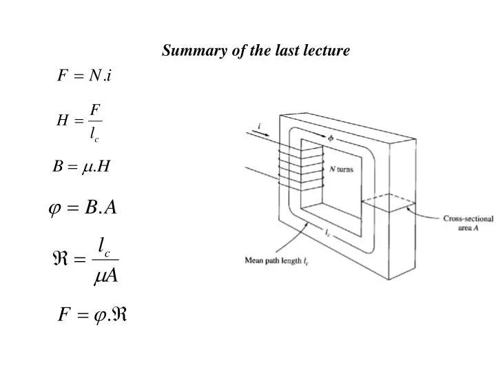
Summary of the last lecture. Magnetic circuits. Compare this formula with Ohm’s law in electric circuits:. Another useful formula in a series situation. Problem 1-8. Assume 4% increase in effective Cross-sectional area for fringing effect. Calculate the flux density in each of the legs.

E N D
Magnetic circuits Compare this formula with Ohm’s law in electric circuits:
Problem 1-8 Assume 4% increase in effective Cross-sectional area for fringing effect Calculate the flux density in each of the legs
Magnetic Behaviour of Ferromagnetic Materials We talked about Ferromagnetic materials, such as iron, steel, cobalt, nickel and some alloys. They have a high relative permeability (2000-6000). In magnetic circuit theory we assumed: where is a constant.
By this assumption we have assumed a linear relation, i.e.: This means in a coil if I increase the current to twice as much, the flux will be twice as much as well. This is what we call linear relation.
But the reality is different. These are typical curves.We have saturation.
Now, can we solve the problems knowing these curves ? In some problems, instead of giving the relative permeability, they produce the B-H curve. In these cases, the operating condition (Bo-Ho), should be known somehow. If it is known, there would be no problem.
Remember the example: Given : i=1 A, N=100, lc=40 cm, A= 100 cm2 r =5000 Calculate : F, H, B, , and
Now consider this example: Given : i=1 A, N=100, lc=40 cm, A= 100 cm2 given the above B-H curve Calculate : F, H, B, , and From the magnetizing curve:
Hysteresis When we increased the current we observed, saturation. What would happen if I decrease the current after saturation? The flux for a given H is higher when decreasing
Can we explain the hysteresis phenomena? All materials consist of small magnetic domains. When they are in a magnetic field the domains are intended to be in line with the field.
The domains after applying magnetic field The domains before applying magnetic field When the magnetic field is removed, not all domains are randomized again
Hysteresis loss Hysteresis is not a serious problem when we have DC excitation (the examples considered so far). It causes some loss when we have AC excitation, called hysteresis loss. If we have AC excitation, e.g. the current i is sinusoid, the hysteresis happens at each cycle. The hysteresis loss is proportional to the frequency and also depends on the area of the hysteresis loop.
Other losses - Copper loss: - Eddy Current loss: - Core losses:
Eddy Current Eddy current: As we saw, a flux induces a voltage on a coil. Q: Why not inducing a voltage on the core itself? A: It actually does. The result is eddy current. That is why the transformers core are laminated.