Download

1 / 30
300 likes | 415 Views
Statistics 102. Outline. I. Sensitivity and Specificity/Likelihood Ratios II. Statistical significance for group data III. Statistical significance for correlational data IV. Non-inferiority trials V. Linear regression VI. Logistic regression VII. Stepwise multivariate regression

E N D
Outline I. Sensitivity and Specificity/Likelihood Ratios II. Statistical significance for group data III. Statistical significance for correlational data IV. Non-inferiority trials V. Linear regression VI. Logistic regression VII. Stepwise multivariate regression VIII. Type I and II errors/ Sample size estimates
I. Sensitivity and Specificity • Sensitivity: true positives (proportion of individuals with the disease who test +; ranges from 0 to 1, or from 0% to 100%) • 1-Sensitivity: false negatives (proportion of individuals with the disease who test -; ranges from 0 to 1, or 0% to 100%) • If sensitivity = 0.8 (80%), 1-sensitivity = 0.2 (20%) • Specificity: true negatives (proportion of individuals without the disease who test -; ranges from 0 to 1, or from 0% to 100%) • 1-Specificity: false positives (proportion of individuals without the disease who test +; ranges from 0 to 1, or 0% to 100%) • If specificity = 0.92 (92%), 1-specificity = 0.08 (8%)
Use of Sensitivity and 1-Specificity in Receiver Operating Curves (ROCs) and the Areas under the ROCs (the AUC) • Plots sensitivity of the test (true + rate, TPR) on Y axis, from 0 to 1 vs. 1-specificity (false + rate, FPR) on X axis, from 0 to 1 at different test cutoffs • Perfect Classification: AUC=1 (area of a square with sides=1) • Random guess: AUC=0.5 (area of a triangle with base and height=1) • AUC between 0.5 and 1: Test is Better than a random guess • AUC between 0 and 0.5: Test is Worse than a random guess • AUC has a 95% CI • e.g., 0.78 (0.69-0.87)
ROCs with AUCs better than a random guess (between 0.5 and 1.0) ↓ = “sweet spot” cut off, a trade off between sensitivity and specificity High cut off →→→→→→→→→→→→→→→ Low cut off
Additional terms that can be derived from sensitivity and specificity • Likelihood ratios: does the test usefully change the probability (likelihood) of a disease or condition? • Positive likelihood ratio= true+/false + =sensitivity/1-specificity. • The higher the + likelihood ratio, the more confident we are that the patient has the condition if the test is +. + LR can approach . • Negative likelihood ratio = false-/true - = 1- sensitivity/ specificity. • The lower the – likelihood ratios, the more confident we are that the patient does not have the condition if the test is -. – LR can approach 0.
Example 1: Use of + and - likelihood ratios • Your patient with COPD has an acute onset of worsening dyspnea. He had arthroscopic knee surgery 2 weeks ago. There is no leg swelling or leg pain, hemoptysis, personal or family history PE or DVT, or malignancy. You clinically assess the odds of him having a PE as 50:50, or equally likely that he had a PE as that he did not have a PE. • If ordered and performed, how would the results of a CT angiogram (CTA) of the pulmonary arteries change your estimated likelihood of PE in this patient? In other words, how good is CTA in helping you diagnose or exclude a PE in this patient?
Example 1, continued Literature (Annals Internal Medicine 136: 286-287, 2002): CTA and pulmonary angiography (gold standard) were performed in 250 patients with possible PE. 50 (20%) of the patients had PE on pulmonary angiography. 200 had no PE on angiography. Results: CTA+CTA- PE on pulm angio (n=50) 35 15 No PE on pulm angio (n=200) 2 198
Example 1, continued Likelihood ratio (LR) calculations: CTA sensitivity (true +)= 35/50 (.70) , or 70% 1-sensitivity (false - )= 15/50 (.30) CTA specificity (true - )= 198/200 (.99), or 99% 1-specificity (false + )=2/200 (.01) +LR = sensitivity/1-specificity = true+/false+ = .70/.01=70 (PE 70 x as likely as before test). -LR = 1-sensitivity /specificity= false-/true- = .30/.99=.303 (PE .3 x as likely as before test) Annals Internal Medicine 136: 286-287, 2002
II. Are measured group differences in variables or outcomes statistically significant? Which test(s) to use? • If data are normally distributed: • Use paired t (if each subject is his/her own control) 1 • Use unpaired t (group t) if there are two groups 2 • If data are skewed (not normally distributed): • Is the variable a continuous one, such as age or PaO2? • Use Mann Whitney U, 3, or • Use Wilcoxon’s sign rank 4 • Is the variable a categorical one, such as gender or age > 65? • Use Fisher’s exact, 5, or • Use chi square test 6 • If there >2 study groups: • Use analysis of variance (ANOVA) 7
If the variables are normally distributed: Use Pearson’s test 8: Pearson’s r ranges from -1 to +1. r 0 indicates no correlation. P value depends both on r and N. If the variables are skewed (not normally distributed): Use Spearman’s test 9: Spearman’s r ranges from -1 to +1 r 0 indicates no correlation. P values depend both on r and N. P< 0.05 usually used. III. Are correlations between variables statistically significant? What test(s) to use?
IV. Non-Inferiority Trials A New Treatment Can Truly Be: • Better (Superior) • Essentially equal • Worse (Inferior) than the usual treatment A Trial Can Test Whether New is: • Better (superior) • Not better (non-superior)* • Not worse (non-inferior) • Worse (Inferior)* * rarely done
Non-inferiority trials • Non-inferiority trials are intended to show that the effect of a new treatment is not worse than that of an active control by more than a specified amount. • A little like a point spread in football. • The non-inferiority margin (NIM) is chosen by the investigators before the study (a priori) and can be somewhat arbitrary. • Study endpoints in non-inferiority trials can be efficacy or safety parameters or a combination of the two. • Study design may include 3 arms with placebo group (preferred) or 2 arms with only new and usual treatments (much less ideal, since no internal validation that new treatment is better than placebo) • Delta (δ) is the measured difference (best estimate of the true difference) between the two active treatments. This δ will have a 95% CI. • Example 3: δ = -4% (95% CI, -9% to +1%)
Example 3: δ = -4% (95% CI, -9% to +1%), the control Rx being slightly better • If the NIM had been chosen to be -10 % by the investigators a priori, using Example 3, the new drug would be shown to be ‘non-inferior’ to the control, as -10 %, the NIM, was less that the 95% CI for δ, -9% to +1%. • (If the NIM had been chosen to be -5 % by the investigators a priori, using Example 3, the new drug would not be shown to be ‘non-inferior- to the control, as -5%, the NIM, fell in the 95% CI for δ, -9% to +1%. In this context, non-inferiority not shown is the same as being inferior.)
Simple regression: y=mx+b one independent variable, x one dependent variable, y If x=0, y=b, the intercept b can be +, as shown, zero, or – V. Linear regression • • • ∆y /∆x= m, slope y, dep variable • • b x, indep variable
Simple regression: y=mx+b one independent variable, x one dependent variable, y If x=0, y=b, the intercept b can be +, as shown, zero, or - More complex regression: y=m1x1+m2x2+b two independent variables one dependent variable If x1=x2=0, y=b, the intercept b can be +, zero, or - V. Linear regression
VI. Logistic regression. A popular method • A model predicting the probability of a dependent categorical outcome, such as death, using 2 or more patient-specificindependent variables. • The logit, z, is the total contribution of ALL the patient-specific independent variables used in the model to predict the outcome, f(z), the dependent variable. • z=β0+β1x1+β2x2+…+ βnxn. • β0= intercept • β1, β2, … βn are regression coefficients for x1,x2, ... xn • If x1, x2, …,xn all =0 (the pt has no risk factors), z=β0=the risk of the dependent outcome (such as death) when no factors affecting risk are present.. • If βn > 0, then the variable, n, increases the risk of the outcome. • If βn<0, then the variable, n, reduces risk of the outcome. • Large βn means the variable, n, has a large influence on the outcome. • Small βn means the variable n has a small influence on the outcome • f(z)= likelihood of outcome, such as death= ez/(ez+1)= 1/(1+e-z)
The logistic function is useful because it can input any z from + to - whereas the output, f(z), will be confined to values between zero and 1. Note: if z=0, f(z)=0.5, because 1/1+e-0=1/1+1=1/2=0.5
Example 4. Logistic regression. • Three independent variables , x1, x2, and x3 are studied to try to predict the 10-year death risk from heart disease. Using data obtained from a large study population, the following logistic regression model was derived to best fit the data: z=β0+β1x1+β2x2+ β3x3 • x1= age in years above 50 (age is a continuous variable); β1= +2.0 • x2= sex, where 0 is male and 1 is female (gender is a categorical variable);β2= -1.0 • x3= blood cholesterol in mmol/L above 5 mmol/L (194 mg/dL); β3=+1.2 • β0= -5.0. • Risk of death=f(z)=1/(1+e-z), where z (the logit)= -5.0+2.0 x1 - 1.0 x2 + 1.2 x3. • Thus, in a 50 y.o. female with a cholesterol of 5 mmol/L, z=0=-5.0 (see prev Fig)
Logistic regression. • Three independent variables , x1, x2, and x3 are studied to try to predict the 10-year death risk from heart disease. Using data obtained from a large study population, the following logisitic regression model was derived to best fit the data: z=β0+β1x1+β2x2+ β3x3 • x1= age in years above 50 (age is a continuous variable); β1= +2.0 • x2= sex, where 0 is male and 1 is female (gender is a categorical variable);β2= -1.0 • x3= blood cholesterol in mmol/L above 5 mmol/L (194 mg/dL); β3=+1.2 • β0= -5.0. • Risk of death=f(z)=1/(1+e-z), where z (the logit)= -5.0+2.0 x1 - 1.0 x2 + 1.2 x3. • Thus, in a 50 y.o. female with a cholesterol of 5 mmol/L, z=0=-5.0 • Example 4: What is the risk of death in the next 10 years from heart disease in a 50 year man with a blood cholesterol of 7 mmol/L (272 mg/dL)? • z= -5.0+2(50-50) -1(0)+1.2(7-5). Thus, z= -5.0+0+0+2.4= -2.6 • Since z= -2.6 in this man, f(z)=his risk of 10-year death from heart disease = 1/(1+e-z) = 1/(1+e2.6 ) = 0.07, a 7% 10-yr risk. • The 95% confidence intervals can also easily be calculated for f(z).
VII. Stepwise multivariate regression • If several variables, INDIVIDUALLY, help to predict an outcome by univariate analysis, but these variables could be closely related to each other, stepwise multivariate analysis helps sort out independent contributions of the variables. • e.g., blood pressure, BMI and type 2 DM EACH increase risk of MI • This procedure is used primarily in regression modeling. At each step, after a new variable is added, a test is made to see if some variables can be deleted without appreciably increasing the discrepancy between the data and the regression model. • The procedure terminates when the measure is maximized or when the available improvement (by adding more variables) falls below some critical, predetermined value.
Example 5. Stepwise multivariate regression. • Cohort of 300 outpatients with low serum TSH undergoing radioiodine uptake and scan. • Many, but not all, had thyroid disease (e.g., Grave’s). Numerous variables were examined to see which correlated with a normal uptake and scan result. • Three of the numerous variables examined predicted a normal uptake and scan : • If patient was using a statin: OR= 6.5 (95% CI, 2.9-14.6) • If patient was a man: OR= 2.5 (95% CI, 1.3-4.5) • If patient was > 45 years of age: OR= 2.0 (95% CI, 1.1-3.6) • Which of these variables independently predicted a normal thyroid uptake and scan despite the low serum TSH? • Is it statin use, being male, and/ or being older than predicts normal thyroid function if a patient has low serum TSH?
Example 5: Stepwise multivariate regression from Yandell et al. Thyroid 2008; 18:1039-42.
VIII. Type 1(α) and Type 2 (β) Errors Null Hypothesis: there is no differences between two treatments tests Reject the null hypothesis Accept null hypothesis Correct decision (no error) Error Correct decision (no error) Error Type 1 () error (P), which can be large or small Type 2 () error, which can large or small
Choosing the size of and errors • The type 1 error, or (also called P) is conventionally set at 0.05 (5%) • i.e, chance of a type 1 error if the null hypothesis is rejected is < 5% • Can state “p<0.05” or give exact p value (e.g., p=0.001, or p=0.049) • The type 2 error, or , is often set at 2 to 4 times , or 0.10-0.20 (10%-20%) • i.e., chance of making a type 2 error if the null hypothesis is accepted is 10-20% • Power to detect a real difference (and thus to reject the null hypothesis ) = 1- • smaller (e.g., 0.1), more power (.9) • larger (e.g., 0.2), less power (.8) • If a study is highly powered and the null hypothesis is accepted, the chance of there being a true difference is quite small. • If the study is under-powered and the null hypothesis is accepted, there can be little confidence that a true difference has been excluded.
Example 6: Use of α and β in sample size planning A new antibiotic is developed for C. difficile. How many patients would be needed to be included in a phase 3 trial to be able to show that this new drug is superior to metronidazole? To answer this question, we need to know: 1. What is the expected success rate for metronidazole? [P1] 2. What would be a clinically important and expected improvement in success rate (based on phase 1/2 studies) with the new drug? [P2] 3. What should be the (type 1 error) and the (type 2 error) for the study? (Recall: Power = 1- .)
Sample size estimation, cont’d • P1 = 0.75 (metronidazole, based on literature) P2 = 0.90 (New Rx, based on small phase 1/2 trials) = 0.05 (1 in 20) = 0.10 (1 in 10). Power = 0.90 (9 in 10) • Needed N1 and N2 = 158 per group (from Fleiss tables), or 316 patients in total • If 10% drop out rate is expected, then 158+16=174 per group, or 348 patients in total would need be randomized. (This sample size may necessitate a multi-center study to enroll sufficient patients during the proposed time frame.) • Analyze data by intent-to-treat and by evaluable patients.