Download
1 / 19
290 likes | 749 Views
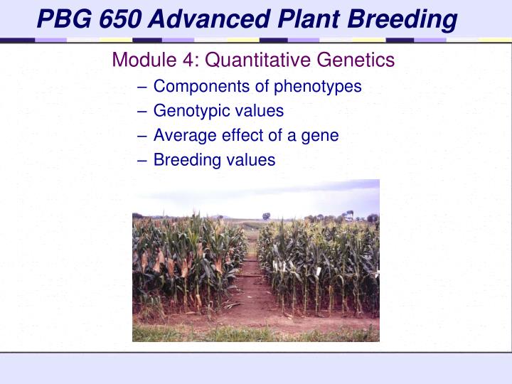
PBG 650 Advanced Plant Breeding. Module 4: Quantitative Genetics Components of phenotypes Genotypic values Average effect of a gene Breeding values. What is Quantitative Genetics?. Definition:

E N D
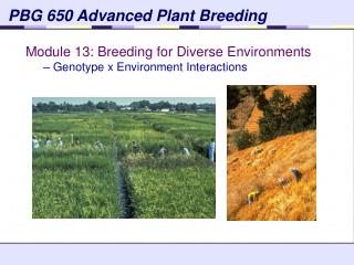
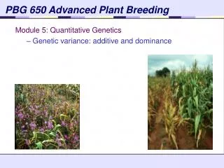
PBG 650 Advanced Plant Breeding Module 4: Quantitative Genetics • Components of phenotypes • Genotypic values • Average effect of a gene • Breeding values
What is Quantitative Genetics? Definition: “Statistical branch of genetics based upon fundamental Mendelian principles extended to polygenic characters” Primary goal: To provide us with a mechanistic understanding of the evolutionary process Lynch and Walsh, Chapter 1
Questions of relevance to breeders • How much of the observed phenotypic variation is due to genetic vs environmental factors? • How much of the genetic variation is additive (can be passed on from parent to offspring)? • What is the breeding value of the available germplasm? • Are there genotype by environment interactions? • What are the consequences of inbreeding and outcrossing? What are the underlying causes? • Are there genetic correlations among traits?
Questions of relevance to breeders • Answers to these questions will influence • response to selection • choice of breeding methods • choice of parents • optimal type of variety (pureline, hybrid, synthetic, etc.) • strategies for developing varieties adapted to target environments
Phenotypic Value P = phenotypic value G = genotypic value E = environmental deviation Components of an individual’s Phenotypic Value P = G + E For individual k with genotype AiAj P(ij)k= + gij + e(ij)k For the population as a whole: E(E) = 0 = E(P) = E(G) Cov(G, E) = 0 Bernardo, Chapt. 3; Falconer & Mackay, Chapt. 7; Lynch & Walsh, Chapt. 4
The origin ( ) is midway between the two homozygotes Single locus model A2A2 A1A2 A1A1 z z+a+d z+2a Genotypic Value Coded Genotypic Value -a 0 d a no dominance d = 0 partial dominance0 <d < +a or0 >d > –a complete dominance d = +aor –a overdominanced > +a or d < –a degree of dominance =
Single locus model Different scales have been used in the literature A2A2 A1A2 A1A1 -a 0 d a Falconer 0(1+k)a 2a Lynch & Walsh Comstock and Robinson (1948) 0 au a 0a 2a+d Hill (1971) Conversions can be readily made
Population mean M =p2a + 2pqd – q2a =a(p2 – q2) + 2pqd = a(p +q)(p -q) + 2pqd =a(p -q) + 2pqd Mean on coded scale (centered around zero) This is a weighted average contribution from homozygotes and heterozygotes Mean on original scale
=P +a(p -q) + 2pqd Population mean M =a(p -q) + 2pqd When there is no dominance a(p -q) When A1 is fixed a When A2 is fixed -a Potential range 2a If the effects at different loci are additive (independent), then M =Σa(p -q) + 2Σpqd
=P+a(p -q) + 2pqd F2=P+(1/2)d BC1(A1A1)=P+(1/2)a + (3/8)d For ½ A1A1, ½ A1A2 =P+½(a + d) For ½ A1A2, ½ A2A2 = P+½(d - a) BC1(A2A2)=P-(1/2)a + (3/8)d Means of breeding populations In an F2 population, p = q = 0.5 In a BC1 crossed to the favorable parent, p = 0.75, so after random mating In a BC1 crossed to the unfavorable parent, p = 0.25, so after random mating
Average effects • We have defined the mean in terms of genotypic values • Genes (alleles), not genotypes, are passed from parent to offspring • Average effect of a gene (i) • mean deviation from the population mean of individuals who received that gene from their parents (the other gene taken at random from the population) subtract M =a(p -q) + 2pqd
Average effect of a gene substitution Average effect of changing from A2 to A1 = 1 - 2 • a and d are intrinsic properties of genotypes • 1, 2, and are joint properties of alleles and the populations in which they occur (they vary with gene frequencies) q[a+d(q-p)] – (-p)[a+d(q-p)] =a+d(q-p) Average effect of changing from A1 to A2 = - Relating this to the average effects of alleles: 1 = q 2 = -p
Breeding Value Breeding value of individual Aij = i + j • For a population in H-W equilibrium, the mean breeding value = 0 • The expected breeding value of an individual is the average of the breeding value of its two parents • For an individual mated at random to a number of individuals in a population, its breeding value is 2 x the mean deviation of its progeny from the population mean.
Regression of breeding value on genotype Breeding values • can be measured • provide information about genetic values • lead to predictions about genotypic and phenotypic values of progeny Additive genetic variance • variance in breeding values • variance due to regression of genotypic values on genotype (number of alleles) ● genotypic value ○breeding value
Genotypic values • Genotypic values have been expressed as deviations from a midparent • To calculate genetic variances and covariances, they must be expressed as a deviation from the population mean, which depends on gene frequencies subtract M =a(p -q) + 2pqd Remember = a + d(q - p) Substitute a= - d(q - p)
Dominance deviation Components of an individual’s Phenotypic Value P = G + E G = A + D • In terms of statistics, D represents • within-locus interactions • deviations from additive effects of genes • Arises from dominance between alleles at a locus • dependent on gene frequencies • not solely a function of degree of dominance • (a locus with completely dominant gene action contributes substantially to additive genetic variance) Gij = + i +j + ij
Partitioning Genotypic Value When p = q = 0.5 (as in a biparental cross between inbred lines)
-2q2d 2pqd -2p2d Dominance deviations from regression
Interaction deviation • Components of an individual’s Phenotypic Value P = G + E P = A + D + E • When more than one locus is considered, there may also be interactions between loci (epistasis) G = A + D + I P = A + D + I + E • ‘I’ is expressed as a deviation from the population mean and depends on gene frequencies • For a population in H-W equilibrium, the mean ‘I’ = 0