Download
1 / 39
410 likes | 648 Views
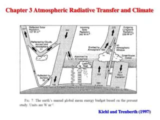
Lecture 3 Radiative Transfer. Lower Solar Atmosphere has two layers: Photosphere - 100 km thick; opaque Chromosphere - 10,000 km thick; optically thin; cooler. (I) Local Thermodynamic Equilibrium Equation of Transfer: Optical Depth. Thermodynamic Equilibrium

E N D
Lower Solar Atmosphere has two layers: • Photosphere - 100 km thick; opaque • Chromosphere - 10,000 km thick; optically thin; cooler
(I) Local Thermodynamic Equilibrium • Equation of Transfer: • Optical Depth
Thermodynamic Equilibrium • A single value of temperature T is sufficient to describe the thermodynamic state everywhere • state of excitation is governed by Boltzman equation • state of ionization is governed by Saha equation • radiation field is homogeneous and isotropic black body
Local Thermodynamic Equilibrium (LTE) Above conditions are satisfied in a local area. Such conditions are usually satisfied in the continuum of visible and near infrared, and wings of most spectral lines
The key is to find two quantum mechanics quantities , in the expression of a, damping constant and f, the oscillator strength in addition Doppler width is modified in the existence of turbulence velocity
Non-LTE: Statistical Equilibrium Temperature is now defined as electron temperature, Te , velocity distribution is still Maxwellian, because of frequent collision.
Einstein Coefficients Considering a line radiation between two energy levels EL (lower) and EU (upper), h= EU-EL • Spontaneous emission from upper to lower energy nU AUL()/4number of emissions per unit time, volume, frequency interval and solid angle.nU : number of atoms in upper level/volume;(): frequency distribution of emitted photon;AUL: Einstein coefficient for spontaneous emission (It’s dimension is 1/time; 108 s-1 is typical.)
Induced Emission and AbsorptionnU BULI()/4 emissionnU BLUI()/4 absorptionI : radiation intensity;(): line profile;BUL and BLU : Einstein coefficient of induced emission and absorption.B, I have the same unit as A.
Continuum Radiation • PhotoionizationNumber of photoionizations from level j, unit time, volume, frequency interval and solid angle: • Radiative Recombination
Collisioncollision transition rate: Cij, which has no direct influence on radiation field, could be for line transition or continuum transition.
Model Calculation of LTE (Fig 4.4) • Usually, we select =5000 Angstrom as a reference wavelength as it is free of absorption line.For LTE, we have S=B ,fromB , we derive T()
Non-LTEAt temperature minimum T=4200 K, 5000=10 -4,LTE model is no longer applicable.Reason is that photo-ionization dominates over radiative recombination, i.e., neutral population is lower.Figs 4.7 & 4.8 give an example for SiI.Two famous models: • HSRA: Harrard-Smithsonian Reference atmosphere Gingerich et al. (1971) Solar Physics, 18, 347 • VAL model: Vernazza, Avrett and Loeser 1976, Ap.J Supp. 30. 1981, Ap.J Supp. 45, 635
Fig 4.9, Fig 4.10The models here are called semi-empirical as T is adapted in order to reproduce observed intensity I.Table 4.1 Special Lines: H line D3 and He I 10830 line CaII H and K lines A Simple Atmosphere Model: S is constant =B
Forbidden lines Violates selection rule, so normally the radiative probability is much smaller than the collisional de-excitation, but in the corona, the opposite is true. Resonant Lines (Strong lines, such as H and K) Equivalent Width Integrated Line Intensity Curve of Growth Equivalent Width (W) as a function of number of absorbing atoms (N). It is used to determine abundance and temperature. For weaker lines, W is proportional to N For strong lines, W is proportional to N 1/2
Chemical CompositionChemical composition can be derived from spectrum analyses - Spectrum Synthesis • Standard Symbol: log A = 12 + log(ni/nH) ni=1012 particle/unit volume Table 4.2 • Helium: It was discovered in 1868 by Lockyer. Most accurate determination of Y is from inversion of helium seismology. Y = 0.248 +/- 0.002 • Lithium depletion: due to burning of lithium at T=2.510 6 K, t = 5 107 yrs.
HW Set # 3 • Problems 4.1, 4.2, 4.4, 4.10