Download
1 / 99
1.38k likes | 1.99k Views
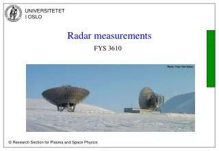
Radar Measurements II. Chris Allen (callen@eecs.ku.edu) Course website URL people.eecs.ku.edu/~callen/725/EECS725.htm. Ground imaging radar. In a real-aperture system images of radar backscattering are mapped into slant range, R, and along-track position.

E N D
Radar Measurements II • Chris Allen (callen@eecs.ku.edu) • Course website URL people.eecs.ku.edu/~callen/725/EECS725.htm
Ground imaging radar • In a real-aperture system images of radar backscattering are mapped into slant range, R, and along-track position. • The along-track resolution, y, is provided solely by the antenna. Consequently the along-track resolution degrades as the distance increases. (Antenna length, ℓ, directly affects along-track resolution.) • Cross-track ground range resolution, x, is incidence angle dependent • where p is the compressed pulse duration • slant range • slant range • along-track • direction • y • R • cross-track • direction • ground range • ground range • x • cross-track • direction • x
Slant range vs. ground range • Cross-track resolution in the ground plane (x) is theprojection of the range resolution from the slant planeonto the ground plane. • At grazing angles ( 90°), r x • At steep angles ( 0°), x • For = 5°, x = 11.5 r • For = 15°, x = 3.86 r • For = 25°, x = 2.37 r • For = 35°, x = 1.74 r • For = 45°, x = 1.41 r • For = 55°, x = 1.22 r
Real-aperture, side-looking airborne radar (SLAR) image of Puerto Rico • ~ 40 x 100 miles • Mosaicked image composed of 48-km (30-mile) wide strip map imagesRadar parametersmodified Motorola APS-94D systemX-band (3-cm wavelength)altitude: 8,230 m (above mean sea level)azimuth resolution: 10 to 15 m • Digital Elevation Model of Puerto Rico
Another SLAR image • 5-m (18 feet) SLAR antenna mounted beneath fuselage • SLAR image of river valley • SLAR operator’s console • X-band system • Civilian uses include: • charting the extent of flood waters, • mapping, locating lost vessels, • charting ice floes, • locating archaeological sites, • seaborne pollution spill tracking, • various geophysical surveying chores.
Limitations of real-aperture systems • With real-aperture radar systems the azimuth resolution depends on the antenna’s azimuth beamwidth (az) and the slant range, R • Consider the AN/APS 94(X-band, 5-m antenna length) az = 6 mrad or 0.34 • For a pressurized jet aircraft • altitude of 30 kft (9.1 km) and an incidence angle of 30 for a slant range of 10.5 km • R = h/cos = 9100 / cos 30 = 10500 m • y = 63 m(coarse but useable) • Now consider a spaceborne X-band radar (15-m antenna length) az = 2 mrad or 0.11 • 500-km altitude and a 30 incidence angle (27.6 look angle) for a 570.5-km slant range • y = 1.1 km(very coarse) • The azimuth resolution of real-aperture radar systems is very coarse for long-range applications
Radar equation for extended targets • Since A = x y we have • Substituting these terms into the range equation leads to • note the range dependence is now R-3 whereas for a point target it is R-4 This is due to the fact that a larger area is illuminated as R increases.
SNR and the radar equation • Now to consider the SNR we must use the noise power • PN = kT0BF • Assuming that terrain backscatter, , is the desired signal (and not simply clutter), we get • Solving for the maximum range, Rmax, that will yield the minimum acceptable SNR, SNRmin, gives
Radar altimetry • Altimeter – a nadir-looking radar that precisely measures the range to the terrain below. The terrain height is derived from the radar’s position.
Altimeter data • Radar map of the contiguous 48 states.
TOPEX/Poseidon • A - MMS multimission platform B - Instrument module 1/Data transmission TDRS 2/Global positioning system antenna 3/Solar array 4/Microwave radiometer 5/Altimeter antenna 6/Laser retroreflectors 7/DORIS antenna • Dual frequency altimeter (5.3 and 13.6 GHz) operating simultaneously. • Three-channel radiometer (18, 21, 37 GHz) provides water vapor data beneath satellite (removes ~ 1 cm uncertainty). • 2-cm altimeter accuracy100 million echoes each day10 MB of data collected per day • French-American systemLaunched in 199210-day revisit period (66 orbit inclination)Altitude: 1336 kmMass: ~ 2400 kg
Altimeter data • Global topographic map of ocean surface produced with satellite altimeter.
Mars Orbiter Laser Altimeter (MOLA) • Laser altimeter (not RF or microwave) • Launched November 7, 1996 • Entered Mars orbit on September 12, 1997 • Selected specifications 282-THz operating frequency (1064-nm wavelength) 10-Hz PRF 48-mJ pulse energy 50-cm diameter antenna aperture (mirror) 130-m spot diameter on surface 37.5-cm range measurement resolution
Radar altimetry • The echo shape, E(t), of altimetry data is affected by the radar’s point target response, p(t), it’s flat surface response, S(t), which includes gain and backscatter variations with incidence angle, and the rms surface height variations, h(t). • Analysis of the echo shape, E(t), can provide insight regarding the surface. From the echo’s leading we learn about the surface height variations, h(t), and from its trailing edge we learn about the backscattering characteristics, ().
Signal integration • Combining consecutive echo signals can improve the signal-to-noise ratio (SNR) and hence improve the measurement accuracy, or it can improve our estimate of the SNR and hence improve our measurement precision. • Two basic schemes for combining echo signals in the slow-time dimension will be addressed. • Coherent integration • Incoherent integration • Coherent integration (also called presumming or stacking) involves working with signals containing magnitude and phase information (complex or I & Q values, voltages, or simply signals that include both positive and negative excursions) • Incoherent integration involves working with signals that have been detected (absolute values, squared values, power, values that are always positive) • Both operations involve operations on values expressed in linear formats and not expressed in dB.
Coherent integration • Coherent integration involves the summation or averaging of multiple echo signal records (Ncoh) along the slow-time dimension. • Coherent integration is commonly performed in real time during radar operation. • Coherent integration affects multiple radar parameters. • It reduces the data volume (or data rate) by Ncoh. • It improves the SNR of in-band signals by Ncoh. • It acts as a low-pass filter attenuating out-of-band signals.
Coherent integration • Signal power found using • where vs is the signal voltage vector • Noise power found using • where vs+n is the signal + noise voltage vector • SNR is then • note that [std_dev]2is variance
Coherent integration • SummingNcoh noisy echoes has the following effect • Signal amplitude is increased by Ncoh • Signal power is increased by (Ncoh)2 • Noise power is increased by Ncoh • Therefore the SNR is increased by Ncoh • Noise is uncorrelated and therefore only the noise power adds whereas the signal is correlated and therefore it’s amplitude adds. This is the power behind coherent integration. • AveragingNcoh noisy echoes has the following effect • Signal amplitude is unchanged • Signal power is unchanged • Noise power is decreased by Ncoh • Therefore the SNR is increased by Ncoh • Noise is uncorrelated and has a zero mean value. • Averaging Ncoh samples of random noise reduces its variance by Ncoh and hence the noise power is reduced.
Coherent integration • Underlying assumptions essential to benefit from coherent integration. • Noise must be uncorrelated pulse to pulse. Coherent noise (such as interference) does not satisfy this requirement. • Signal must be correlated pulse to pulse. That is, for maximum benefit the echo signal’s phase should vary by less than 90 over the entire integration interval. For a stationary target relative to the radar, this is readily achieved. For a target moving relative to the radar, the maximum integration interval is limited by the Doppler frequency. This requires a PRF much higher than PRFmin, that is the Doppler signal is significantly oversampled. • Ncoh = 10
Coherent integration • Coherent integration filters data in slow-time dimension. • Filter characterized by its transfer function.
Coherent integration • Impact on SNR • Coherent integration improves the SNR by Ncoh. • For point targets • For extended targets • SNRvid • SNRcoh
Coherent integration • So what is going on to improve the SNR ? • Is the receiver bandwidth being reduced ? No • By coherently adding echo signal energy from consecutive pulses we are effectively increasing the illumination energy. • This may be thought of as increasing the transmitted power, Pt. • Again returning to the ACR 430 airfield-control radar example • The transmitter has peak output power, Pt, of 55 kW and a pulse duration, , of 100 ns, (i.e., B = 10 MHz). • Hence the transmit pulse energy is Pt = 5.5 mJ • Coherently integrating echoes from 10 pulses (Ncoh = 10) produces an SNR equivalent to the case where Pt is 10 times greater, i.e., 550 kW and the total illumination energy is 55 mJ. • Alternatively, coherent integration permits a reduction of the transmit pulse power, Pt, equivalent to the Ncoh while retaining a constant SNR.
Incoherent integration • Incoherent detection is similar to coherent detection in that it involves the summation or averaging of multiple echo signal records (Ninc) along the slow-time dimension. • Prior to integration thesignals aredetected(absolute values, squared values, power, values that are always positive). • Consequently the statistics describing the process is significantly more complicated (and beyond the scope of this class). • The improvement in signal-to-noise ratio due to incoherent integration varies between Ninc and Ninc, depending on a variety of parameters including detection process and Ninc. • How it works: For a stable target signal, the signal power is fairly constant while the noise power fluctuates. Therefore integration consistently builds up the signal return whereas the variability of the noise power is reduced. Consequently the detectability of the signal is improved.
Incoherent integration • Example using square-law detection
More on coherent integration • l = 30 cm • 90 m/s • 1 km • 2 km • Clearly coherent integration offers tremendous SNR improvement. • To realize the full benefits of coherent integration the underlying assumptions must be satisfied • Noise must be uncorrelated pulse to pulse • Signal phase varies less than 90 over integration interval • The second assumption limits the integration interval for cases involving targets moving relative to the radar. • Coherent integration can be used if phase variation is removed first. • Processes involved include range migration and focusing. • For a 2.25-kHz PRF, Ncoh = 100,000 or 50 dB of SNR improvement
Tracking radar • In this application the radar continuously monitors the target’s range and angular position (angle-of-arrival – AOA). • Tracking requires fine angular position knowledge, unlike the search radar application where the angular resolution was el and az. • Improved angle information requires additional information from the antenna. • Monopulse radar • With monopulse radar, angular position measurements are accomplished with a single pulse (hence the name monopulse). • This system relies on a more complicated antenna system that employs multiple radiation patterns simultaneously. • There are two common monopulse varieties • amplitude-comparison monopulse • phase-comparison monopulse • Each variety requires two (or more) antennas and thus two (or more) receive channels
Amplitude-comparison monopulse • This concept involves two co-located antennas with slightly shifted pointing directions. • The signals output from the two antennas are combined in two different processes • (sum) output is formed by summing the two antenna signals • (difference) output is formed by subtracting signals from one another • These combinations of the antenna signals produce corresponding radiation patterns ( and ) that have distinctly different characteristics • / (computed in signal processor) provides an amplitude-independent estimate of the variable related to the angle
Phase-comparison monopulse • This concept involves two antennas separated by a small distance d with parallel pointing directions. • The received signals are compared to produce a phase difference, , that yields angle-of-arrival information. • For small , sin
Dual-axis monopulse • Both amplitude-comparison and phase-comparison approaches provide angle-of-arrival estimates in one-axis. • For dual-axis angle-of-arrival estimation, duplicate monopulse systems are required aligned on orthogonal axes.
Monopulse • Conventional monopulse processing to obtain the angle-of-arrival is valid for only one point target in the beam, otherwise the angle estimation is corrupted. • Other more complex concepts exist for manipulating the antenna’s spatial coverage. • Theses exploit the availability of signals from spatially diverse antennas (phase centers). • Rather than combining these signals in the RF or analog domain, these signals are preserved into the digital domain where various antenna patterns can be realized via ‘digital beamforming.’
Frequency agility • Frequency agility involves changing the radar’s operating frequency on a pulse-to-pulse basis. (akin to frequency hopping in some wireless communication schemes) • Advantages • Improved angle estimates (refer to text for details) • Reduced multipath effects • Less susceptibility to electronic countermeasures • Reduced probability detection, low probability of intercept (LPI) • Disadvantages • Scrambles the target phase information • Changing f changes • To undo the effects of changes in f requires precise knowledge of R • Pulse-to-pulse frequency agility is typically not used in coherent radar systems.
Pulse compression • Pulse compression is a very powerful concept or technique permitting the transmission of long-duration pulses while achieving fine range resolution.
Pulse compression • Pulse compression is a very powerful concept or technique permitting the transmission of long-duration pulses while achieving fine range resolution. • Conventional wisdom says that to obtain fine range resolution, a short pulse duration is needed. • However this limits the amount of energy (not power) illuminating the target, a key radar performance parameter. • Energy, E, is related to the transmitted power, Pt by • Therefore for a fixed transmit power, Pt, (e.g., 100 W), reducing the pulse duration, , reduces the energy E. • Pt = 100 W, = 100 ns R= 50 ft, E = 10 J • Pt = 100 W, = 2 ns R= 1 ft, E = 0.2 J • Consequently, to keep E constant, as is reduced, Pt must increase.
More Tx power?? • Why not just get a transmitter that outputs more power? • High-power transmitters present problems • Require high-voltage power supplies (kV) • Reliability problems • Safety issues (both from electrocution and irradiation) • Bigger, heavier, costlier, …
Simplified view of pulse compression • P1 • t1 • Power • Goal: • t2 • P2 • time • Energy content of long-duration, low-power pulse will be comparable to that of the short-duration, high-power pulse • 1 « 2 and P1» P2
Pulse compression • Radar range resolution depends on the bandwidth of the received signal. • The bandwidth of a time-gated sinusoid is inversely proportional to the pulse duration. • So short pulses are better for range resolution • Received signal strength is proportional to the pulse duration. • So long pulses are better for signal reception • Solution: Transmit a long-duration pulse that has a bandwidth corresponding to that of a short-duration pulse c = speed of light, R = range resolution, = pulse duration, B = signal bandwidth
Pulse compression, the compromise • Transmitting a long-duration pulse with a wide bandwidth requires modulation or coding the transmitted pulse • to have sufficient bandwidth, B • can be processed to provide the desired range resolution, R • Example: • Desired resolution, R= 15 cm (~ 6”) Required bandwidth, B = 1 GHz (109 Hz) • Required pulse energy, E = 1 mJ E(J) = Pt(W)· (s) • Brute force approach • Raw pulse duration, = 1 ns (10-9 s) Required transmitter power, Pt = 1 MW ! • Pulse compression approach • Pulse duration, = 0.1 ms (10-4 s) Required transmitter power, Pt = 10 W
Pulse coding • The long-duration pulse is coded to have desired bandwidth. • There are various ways to code pulse. • Phase code short segments • Each segment duration = 1 ns • Linear frequency modulation (chirp) • for 0 t • fC is the starting frequency (Hz) • k is the chirp rate (Hz/s) • B = k = 1 GHz • Choice driven largely by required complexity of receiver electronics • 1 ns • t
Receiver signal processingphase-coded pulse compression • time • Correlation process may be performed in the analog or digital domain. A disadvantage of this approach is that the data acquisition system (A/D converter) must operate at the full system bandwidth (e.g., 1 GHz in our example). • PSL: peak sidelobe level (refers to time sidelobes)
Binary phase coding • Various coding schemes • Barker codes • Low sidelobe level • Limited to modest lengths • Golay (complementary) codes • Code pairs – sidelobes cancel • Psuedo-random / maximal length sequential codes • Easily generated • Very long codes available • Doppler frequency shifts and imperfect modulation (amplitude and phase) degrade performance
Chirp waveforms and FM-CW radar • To understand chirp waveforms and the associated signal processing, it is useful to first introduce the FM-CW radar. • FM – frequency modulation • CW – continuous wave • This is not a pulsed radar, instead the transmitter operates continuously requiring the receiver to operate during transmission. • Pulse radars are characterized by their duty factor, D • where is the pulse duration and PRF is the pulse repetition frequency. • For pulsed radars D may range from 1% to 20%. • For CW radars D = 100%.