Download

1 / 15
150 likes | 278 Views
Presenter : Monica Farkash Bryan Hickerson mfarkash@us.ibm.com bhickers@us.ibm.com. Regression Optimization using Hierarchical Jaccard Similarity and Machine Learning. Outline. The challenge: Providing a subset from a regression test suite

E N D
Presenter: Monica Farkash Bryan Hickerson mfarkash@us.ibm.combhickers@us.ibm.com Regression Optimization using Hierarchical Jaccard Similarity and Machine Learning
Outline • The challenge: Providing a subset from a regression test suite • Our new Jaccard/K-means (JK) approach • Hierarchical Distance and Jaccard Similarity Index • Clustering • IBM experiences: successful at keeping important test cases in the regression
Validating New Models New model validation Feature Verification New model validation Terminology: Regression test suite • To reduce costs and reduce delay => reduce number tests in regression • Existing solutions: • Empirical: ranking in % coverage • Greedy algorithm • Problems with existing solutions: • Wrong measure to decide (point coverage not paths) • Not a global view (greedy), doesn’t provide an optimized, balanced result Model Release Point Model Release Point Run Regression Tests
“Similar” Machine Learning Solution Our Contribution Replacement Test suite Original Test suite • Replacement test suite has the quality of being the mostsimilar to the initial one. • New definition for similarity: • Hierarchical approach to distance – taking into account all hierarchical layers with common activity • Pseudo-distance between two tests • Different way to measuring the quality of a test: • Path – Hierarchical stimulated HW paths more important than touching certain “end” points, especially for model changes • Quantity of covered monitors differs among units and must be accounted for • New algorithm: machine learning We show results on a real life example
Cluster New Jaccard/K-means (JK) Solution Our new solution has the following steps: 1. Use a similarity index that can provide information on how similar two tests are, meaning how “close” the stimulated HW paths they cover are to each other. 2. Use a clustering algorithm to group the tests into clusters of similar tests, using as “distance” the similarity index defined above. 3. For each cluster, choose a representative test that will replace all the tests from a cluster in the new regression test suite. The new regression test suite is built by putting together a representative test for each cluster. Read Test coverage Compute Test To Test Hierarchical “distance” Choose representatives Original Test suite New Test suite
JK: Similarity as Pseudo-Distance Intuitively, if two tests do ”vey similar things” => they are “close” to each other if two tests do totally different things => they are “different” from each other => We need to measure a distance between two tests • Distance between two tests is determined on how the tests exercise the HW model, not between the tests themselves. • Coverage measures the “impact” a test has on a HW model when run => we can define a pseudo-distance using the coverage they generate • We introduce a new notion of test to test pseudo-distance (TT) and a formula that provides us with a measurable distance between two tests, expressing how close (that is, how similar) the tests are by measuring the correlation between their stimulated HW paths. t1 t1coverage simulation “distance”= similarity t2 t2coverage
t1coverage t2coverage Similar tests though not overlapping coverage JK: HierarchicalSimilarity • Importance of hierarchy: • Current coverage analysis is generally linear; it considers all the monitors as having the same importance regardless where they are in the hierarchy. • HW paths at higher levels are more commonly covered and less relevant in comparing two tests than “deep” areas being covered by both. • We define a similarity index that reflects the hierarchical nature of the distances between t1 and t2 coverage (tests 1 and test 2 ) as follows: di is the distance computed at level i wi is the weight given to the level i in the hierarchical structure TT(t1,t2) = SUM ( wi*di) • The weights are chosen such that they considerably weight the TT value towards overlapping “deep” monitors.
Level 1: 1 Level 2: 1 Level 3: 1/7 t1coverage t1coverage t2coverage t2coverage t1coverage/level t2coverage/level t1coverage t2coverage Similar tests though not overlapping coverage JK: One Level Similarity • At each hierarchical layer we measure: “ rate of common versus all “ • Jaccard similarity coefficient TT(t1,t2) = SUM { wi* [same_further_path(t1ij,t2ij)] / all_paths_further(t1it2i)] } • The similarity is “1” if they are identical at that layer, and “0” if they are disjoint • pseudo-distance=1-similarity
JK: HierarchicalSimilarity: Example The example to the left shows three tests, A,B,C. The similarity index is being provided in the table. We compute the “area” that was commonly covered by two tests. A,B are most similar, even though they share no coverage points while B,C are less similar, even though they share coverage “end” points To help understand how it works in real life, let’s consider the 1st layer of hierarchy as the Instruction Fetch Unit, the 2nd as branch logic, and the 3rd prediction logic. Two tests which do branches might be completely common on H1 as well as H2, but on H3 they differ as one exercises Counter logic and the other exercises testing Control register bits. Similarity might be low as the H3 commonality is low. tAcoverage A tBcoverage B C tccoverage H1 I-Fetch H2 - Branch H3 – conditional on CR H3 – conditional on CTR 9
JK: HierarchicalSimilarity: Real Life Example • We started with a regression test suite containing 100 tests • simulated the test and extracted the coverage • computed the 1x1 pseudo-distances as in the excerpt below. ( 5,000 pseudo-distances ) • The depth of our design is 20 hence each similarity index is computed out of 20 different values, one per “layer” (initial 100,000 distances) • The distances were multiplied with 1000 for easier visibility, in the table below • The distances are portable from a model to another one, from unit to system level • Coverage and distance need to be computed only once
1. 2.a. 2.b. 3 JK: Clustering 1. We provide the distance matrix d(ti,tj) , i,j = 0..n . 2. There are no other points in space but the n given points. 3. We provide k – the number of tests we want for the new regression. Algorithm k-means: 1. Start with randomly chosen k tests to represent the future k clusters. 2. Repeat until fix point (or given threshold): 2.a. Group the remaining tests around these according to the distance among them. 2.b. For each cluster choose a new representative with the least distance to the rest of the tests within the cluster. 3. Provide the clusters and their representatives.
JK: Clustering Results K 80 70 60 50 40 30 20 10 K 80 70 60 50 40 30 20 10 • We ran the clustering algorithm for k =80,70,…,10. The resulting regression suite has the corresponding number of tests. • There is a large variation in the number of tests per cluster. For 10 clusters, their size ranges from 19 tests per cluster (cluster #9) to 3 (#5) • We present as an example cluster #9 (for k=10) • Shows the test distribution from 80 – 10 • Largest (19 tests) • Composed of 5 clusters for k=20 • (T96,T14)(T31,T46) versus T10, T22 • Even with k=80 we continue to have up to 4 tests fully clustered together Breaking down a cluster (for k=10) into small clusters while increasing k • The quality of the new test suite is a function of k. The “cluster inner distance” can be used as a measure of how dissimilar the tests that we clustered together end up being. Worse choice (k=10) provides a max “inner” cluster distance of 0.159
JK: Results Analysis • Clusters vs. Outliers • Greedy algorithms tend to keep the tests with higher coverage %, which are tests that exercise the design with the highest # of coverage monitors => implicit bias towards tests that exercise the same highly loaded paths • Clustering removes common tests and rewards outliers • JK is a fine sensor for measuring uniqueness: • Distinct tests starting at k=70 (T10,T22) • Clusters of common tests still identified at k=80 • Outliers targeted for removal • Example: T11 – in the 10% with least coverage & unique starting with k=40 • Coverage driven selection not satisfactory • All tests in our regression had significant coverage overlapping • 10 best tests provide 80% coverage of all 100 tests • No large variations => more difficult to choose according to pure end-point coverage • Impact of high density versus low density areas • Un-fair coverage points distribution; Reflects the designer not the functionality • Clusters analysis shows they tend to share monitor “density” • Same path => goes to same areas => same “density” of monitors
JK: Summary and Future Work • We approached the problem of reducing the number of tests required for validation by: • Defining a “distance” between two tests that reflects a hierarchical view of coverage and using a Jaccard similarity index based pseudo-distance per hierarchical layer • Clustering the tests to reflect high similarity among them • Choosing from each cluster the most significant test • We applied the solution on a real life application: • Easily identified distinct cases; Optimal for tests with low coverage and unique paths • The solution is not influenced by the variation in density of coverage monitors • JK’s advantages: • Answers better the challenge, by identifying and keeping distinct tests in the suite • Reduced cost => Reduces validation testing costs • Distance computation O( #layers. #coverage points) • K means – O( k. n. #iterations). • Can be ported with the tests from unit to core to system testing JK: Future Work: • Research innovative metrics as mandatory base for data analytic solutions in the EDA field • Extend the use of the JK distance to other applications (e.g. triage and debug support )
References Acknowledgments Prof. Adnan Aziz, UT, Austin, for technical guidance. • Alessandro Orso, Nanjuan Shi, and Mary Jean Harrold. 2004. Scaling regression testing to large software systems. SIGSOFT Softw. Eng. Notes 29, 6 (October 2004), 241-251. • S. Yoo and M. Harman. 2012. Regression testing minimization, selection and prioritization: a survey. Softw. Test. Verif. Reliab. 22, 2 (March 2012), 67-120. • Dawei Qi, Abhik Roychoudhury, Zhenkai Liang, and Kapil Vaswani. 2009. Darwin: an approach for debugging evolving programs. In Proceedings of the the 7th joint meeting of the European software engineering conference and the ACM SIGSOFT symposium on The foundations of software engineering (ESEC/FSE '09). ACM, New York, NY, USA, 33-42. • H. Finch. Comparison of Distance Measures in Cluster Analysis with Dichotomous Data. Journal of Data Science (2005) Volume: 3, Issue: 1, Pages: 85-100 • Christopher M. Bishop. Pattern Recognition and Machine Learning. Springer Verlag 2006. • B. Wile. J. Goss, W. Roesner. Comprehensive Functional Verification. Morgan Kaufmann 2005