Download
1 / 16
160 likes | 262 Views
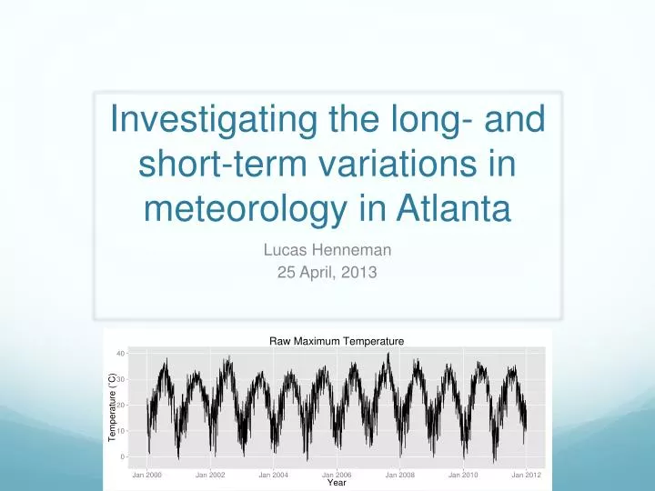
Investigating the long- and short-term variations in meteorology in Atlanta. Lucas Henneman 25 April, 2013. Motivation. Negative health outcomes due to high levels of air pollution have been addressed by enacting regulations on polluters

E N D
Investigating the long- and short-term variations in meteorology in Atlanta Lucas Henneman 25 April, 2013
Motivation • Negative health outcomes due to high levels of air pollution have been addressed by enacting regulations on polluters • Industry, researchers, and policy-makers are interested in the effectiveness of these regulations • Statistical techniques can be used to separate changes in air quality due to emissions from changes due to meteorological fluctuations
Objectives • Compare methods for isolating variations at specific frequencies in a daily time series of maximum temperature • Use these results to remove fluctuations in measured gas-phase pollutant concentrations caused by meteorology
Approach A daily gas-phase species concentration signal can be decomposed into 5 elements as follows: Similarly, a daily meteorological signal can be decomposed into 4 elements: LT: long-term (>365 days) S: seasonal and long meso-scale (30–365 days) W: weekly–present only in pollutant signal (7 days) STM: short-term meteorological (<30 days) WN: white-noise (~1 day)
Data Temperature from the Jefferson Street monitoring station in downtown Atlanta Time period: January 2000 – December 2011 Max Temperature used for a daily metric Less than 10% blank values in the Jefferson Street data, estimated with linear interpolation
Mean Year Method • Adapted from Kuebler et al. (2002). • Long-term (LT) component is captured with the Kolmogorov-Zurbenko (KZ) filter, (365-day averaging window passed three times) (Rao & Zurbenko, 1994) • Seasonal (S) element is captured by averaging each day over the N years of data (here, 12 years) to create a Mean Year (MY), which is smoothed with a local regression loess smoother s[MY(t)] = S(t) • Subtracting LT and S from the original signal yields the daily deviations, or ∆1’s. Signal – LT – MY = STM + WN = ∆1
Fast Fourier Transform Filter Method • Adapted to isolate specific frequencies of variations of meteorological and air pollution signals • LT and S are both removed using the low-pass FFT filter with a cutoff of 30 days (the upper limit of meso-scale meteorology–e.g. hurricanes and fronts) LT + S = FFT>30(Signal) Signal – FFT>30(Signal) = STM + WN = ∆2 • The ∆2’s are regressed against daily deviations in pollution species concentrations to investigate the relationships between meteorology and air pollution.
Examples of FFT filtering www.cd4car.com http://paulbourke.net/miscellaneous/imagefilter/
Spectral Analysis Mean Year Method FFT Method
Spectral Analysis Mean Year Method FFT Method
Conclusions and Future Work • Both methods are effective at removing the annual component of a meteorological signal • Both methods produce ∆’s that are stationary (validated by KPSS hypothesis test) • The Mean Year method imperfectly preserves frequencies below a period of 30 days • The FFT Filter method allows for precise removal of variations at known frequencies
Future Work • Investigate the need for detrending before application of FFT filter (likely not necessary for temperature) • Apply the FFT method to other meteorological and pollution variables to quantify meteorological affect on gas-phase species concentrations • Use the analysis to link higher daily deviations with specific met variables (e.g. ozone with higher incoming solar radiation)
References Duchon, C. and Hale, R. (2012) Fourier Analysis, in Time Series Analysis in Meteorology and Climatology: An Introduction, John Wiley & Sons, Ltd, Chichester, UK. doi: 10.1002/9781119953104.ch1 Kuebler, J., Van den Bergh, H., & Russell, A. G. (2001). Long-term trends of primary and secondary pollutant concentrations in Switzerland and their response to emission controls and economic changes. Atmospheric Environment, 35(8), 1351–1363. doi:10.1016/S1352-2310(00)00401-5 Kwiatkowski, D., P. C. B. Phillips, P. Schmidt and Y. Shin. "Testing the Null Hypothesis of Stationarity against the Alternative of a Unit Root." Journal of Econometrics. Vol. 54, 1992, pp. 159–178. Rao, S., & Zurbenko, I. (1994). Detecting and tracking changes in ozone air quality. Air & waste, 44, 1089–1092. Retrieved from http://www.tandfonline.com/doi/abs/10.1080/10473289.1994.10467303 Stull, R. B. (1988). Ch. 8: Some Mathematical & Conceptual Tools: Part 2. Time Series. Introduction to Boundary Layer Meteorology.