Download
1 / 21
210 likes | 349 Views
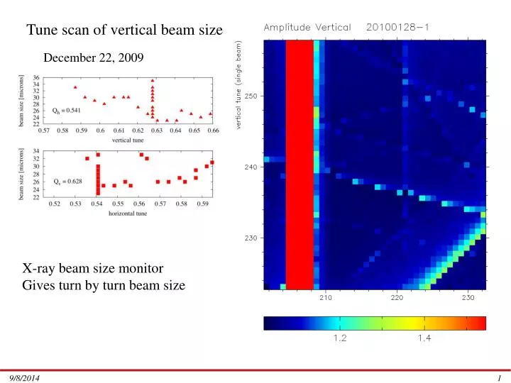
Tune dependence. Tune scan of vertical beam size. December 22, 2009. X-ray beam size monitor Gives turn by turn beam size. Tune dependence. Smallest measured beam size. Largest measured beam size. Cta_2085mev_20090516. Q z =0.066=25.7kHz. nominal. Zero dispersion in RF. Horizontal tune.

E N D
Tune dependence Tune scan of vertical beam size December 22, 2009 X-ray beam size monitor Gives turn by turn beam size
Tune dependence Smallest measured beam size Largest measured beam size
Cta_2085mev_20090516 Qz=0.066=25.7kHz nominal Zero dispersion in RF Horizontal tune Horizontal tune
Qh<0.5 Horizontal tune
Reverse sextupole steering windings - skew quads Skew quad k~0.002/m2 @ 14A
Closed dispersion/coupling bumps ηy at 18-19 η'y at 18-19
BPM systematics Gain mapping
Characterization of BPM Gain Errors Signal at each button depends on bunch current (k) and position (x,y) Signals on the four buttons are related by symmetry Combining sums and differences we find the following relationship, good to second order
Gain characterization simulation Simulation Using a map that reproduces the “exact” dependence of the button signals on the bunch positions we generate B1,B2,B3,B4 for each of 45 points on a 9mm x 5mm grid In first order c=0, and therefore B(+--+) = 0. Evidently the first order approximation is not very good enough this range. The small deviations from the straight line at large amplitudes is a measure of the higher than second order contributions.
Simulation with gain errors Introduce gain errors Zero offset, nonlinearity, and multi - valued relationship i n is a measure of gain errors.
Orbit data collected on a grid To fit for gains Fix g1=1, and minimize with respect to g2,g3,g4,c Fitted gains = 1,0.95,0.96,0.97
Orbit data collected on a grid BPM 75 - fitted gain = 1,1.02,0.96,0.91 BPM 77 - fitted gain = 1,0.92,0.96,0.9 Fit typically reduces 2 by two orders of magnitude
Average gains computed for 6 turn by turn data sets Error bar is the standard deviation of the 6
Fitted gains from 6 turn by turn data sets, RD-000652, 653, 654, 655, 656, 657 Normalized so that average at each BPM of 4 gains is unity Standard deviation, eliminating all points with gain errors greater than 50% is =4.3%
Data from December 19, 2009 • Turn by turn data RD-000908.dat, RD-000909.dat • Immediately followed by • measurement of phase.8607 • and ac_eta.165 • Use turn by turn data to determine gains • Use fitted gains to correct coupling and eta measurements
Summary of fitted gains σ = 4.6%
Coupling without gain correction Coupling with gain correction
Dispersion without gain correction Dispersion with gain correction