Download
1 / 22
220 likes | 504 Views
Hidden Conditional Random Fields. Asela Gunawardana, Milind Mahajan, Alex Acero, John C. Platt Microsoft Research. reference. [ INTERSPEECH 2005 ] Asela Gunawardana, Milind Mahajan, Alex Acero, John C. Platt, “Hidden Conditional Random Fields for Phone Classification”

E N D
Hidden Conditional Random Fields Asela Gunawardana, Milind Mahajan, Alex Acero, John C. Platt Microsoft Research
reference • [INTERSPEECH 2005] Asela Gunawardana, Milind Mahajan, Alex Acero, John C. Platt, “Hidden Conditional Random Fields for Phone Classification” • [ICASSP 2006] Milind Mahajan, Asela Gunawardana, Alex Acero, “Training Algorithm for Hidden Conditional Random Fields”
outline • Introduction • HCRFs as a generalization of HMMs • HCRF estimation • Experimental results • Conclusions
Random Fields • At its most basic a random field is a list of random numbers whose values are mapped onto a space (of n dimensions) • Values in random field are usually spatially correlated in one way or another, in its most basic form this might mean that adjacent values do not differ as much as values that are further apart • Several kinds of random fields exist, among them Markov random fields (MRF), Gibbs random fields (GRF), conditional random fields (CRF), and Gaussian random fields • In detail, please ref: http://en.wikipedia.org/wiki/Random_field
Introduction (1/2) • There has been a resurgence of interest in discriminative methods for ASR due to the success of extended Baum-Welch based techniques such as MMI and MPE training in LVCSR • However, the methods are poorly understood as they are used in ways in which their convergence guarantees no longer hold, and their successful use is as much art as it is science • The rationale for the use of these EBW based techniques is that general unconstrained optimization algorithms are not well-suited to optimizing generative hidden Markov models (HMMs) under discriminative criteria such as the conditional likelihood
Introduction (2/2) • We present a class of models that in contrast to HMMs are discriminative rather than generative in nature, and are amenable to the use of general purpose unconstrained optimization algorithms • The HMM framework is difficult to incorporate long-range dependencies between the states and the observations • Maximum entropy Markov models (MEMMs) are direct (non-generative) models that instead of observations being generated at each state, the state sequence is generated conditioned on the observations
Generative Models • A generative model is a model for randomly generating observed data, typically given some hidden parameters • Generative models are used in machine learning for either modeling data directly (i.e., modeling observed draws from a probability density function), or as an intermediate step to forming a conditional probability density function • Examples of generative models include: • Gaussian distribution • Gaussian mixture model • Multinomial distribution • Hidden Markov model • Generative grammar Ref:http://en.wikipedia.org/wiki/Generative_model
Maximum Entropy Markov Models • The state at each time is chosen with a probability that depends on the previous state as well as the observations • The model does not assign probability to the observations, and the conditional state transition probabilities are exponential (“maximum entropy”) distributions that may depend on arbitrary features of the entire observation sequence P(s|s’,o) that provides the probability of the current state s given the previous state s’ and the current observation o
Conditional Random Fields • CRFs are generalizations of MEMMs where the conditional probability of the entire state sequence given the observation sequence is modeled as an exponential distribution • While MEMMs use per-state exponential distributions to model the transition probability at each state, CRFs use a single exponential distribution to model the entire state sequence given the observation sequence • MEMMs and CRFs have been used successfully for tasks such as part-of-speech (POS) tagging and information extraction
Hidden CRFs • In previous approaches using MEMMs and CRFs for speech, an HMM system is used to reveal the “correct” training state sequence through Viterbi alignment • We generalize this work and use CRFs with hidden state sequences for modeling speech • HCRFs are able to use features which can be arbitrary functions of the observations without complicating the training
HCRFs • CRFs are typically trained using iterative scaling methods or quasi-Newton methods such as L-BFGS • It’s possible to train HCRFs using Generalized EM (GEM) where the M-step is an iterative algorithm such as GIS or L-BFGS, rather than a closed form solution • We have successfully used direct optimization techniques such as L-BFGS and stochastic gradient descent to estimate HCRF parameters
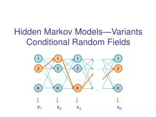
HCRFs vs. HMMs • The key difference between HCRFs and HMMs • HCRFs model the state sequence as being conditionally Markov given the observation sequence • HMMs model the state sequence as being Markov, and each observation being independent of all others given the corresponding state
HCRFs as a generalization of HMMs (1/3) • The HCRF model gives the conditional probability of a segment (phonetic) label ωgiven the observation sequence o = (o1, · · · , oT): λ is the parameter vector and f(w,s,o) is a vector of sufficient statistics referred to as the feature vector. And the partition function z(o; λ) ensures that the model is a properly normalized probability and is given by • The choice of sufficient statistics determines the dependencies modeled by the HCRF
HCRFs as a generalization of HMMs (2/3) • We use the vector of sufficient statistics f with components • These sufficient statistics may be recognized as the ones that are commonly accumulated in order to estimate HMMs • Since all components of f are sums of terms that involve at most pairs of neighboring states
HCRFs as a generalization of HMMs (3/3) • It can be shown that setting the corresponding components of λto Gives the conditional p.d.f. induced by an HMM with transition probabilities , emission means , emission covariance and unigram probability .
HCRF Estimation (1/4) • we have chosen to use direct optimization of the conditional log-likelihood of the training set rather than GEM • Need to find λ to maximize the conditional log-likelihood of the training set • L-BFGS is a batch training method which uses the statistics such as ∇L(λ) computed from the entire training set in order to make an update to the parameter vector λ • Stochastic gradient descent (SGD) updates the parameter vector after processing each single training sample using noisy estimates of the gradient ∇L(λ)
HCRF Estimation (2/4) • If (w(1), o(1)) . . . (w(N), o(N)) is the entire sequence of training samples processed by SGD, then: • where η(n) is the learning rate and U(n) is a conditioning matrix which can be used to speed up the convergence • We used a constant learning rate η(n) = ηandU(n) = I • Both L-BFGS and SGD require the computation of the gradient of numerator denominator
HCRF Estimation (3/4) • The forward and backward recursions and the computation of occupancy probabilities are analogous to the case of HMM estimation, with the transition • probability ass’replaced by a transition score and the observation probability replaced by an observation score
HCRF Estimation (4/4) • Thus, the gradient of the log conditional likelihood can be efficiently computed, just as with MMI estimation of HMMs • Note that the conditional log-likelihood is not convex in λ.Training methods will therefore in general find a local optimum rather than the global optimum. • We initialized the HCRF estimation from ML trained HMM parameters.
Experimental Results Training set: 142910 Development set: 15334 Evaluation set: 7333 It should be noted that while MMI estimation of the HMMs and SGD estimation of the HCRFs converged within ten iterations over the training set, L-BFGS convergence was much slower, taking up to fifty iterations
Conclusions • The advantage of HCRFs is that the model is a state sequence probability model, even when applied to the phone classification task, and can easily be extended to recognition tasks where the boundaries of phonetic segments are unknown • The HCRF framework is easily extensible to recognition since it is a state and label sequence modeling technique • HCRFs have the ability to handle complex features without any change in training procedure