Download
1 / 26
380 likes | 782 Views
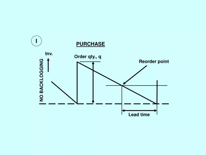
I. PURCHASE. Inv. Order qty., q. Reorder point. NO BACKLOGGING. Lead time. II. PRODUCTION. Inv. q. III. Inv. q. BACKLOGGING. b. IV. Inv. b. WITHOUT BACKLOGGING. C = unit cost (Rs/piece) C 1 = i X C = carrying cost (Rs/unit/time)

E N D
I PURCHASE Inv. Order qty., q Reorder point NO BACKLOGGING Lead time
II PRODUCTION Inv. q
III Inv. q BACKLOGGING b
IV Inv. b
WITHOUT BACKLOGGING C = unit cost (Rs/piece) C1 = i X C = carrying cost (Rs/unit/time) C2 = shortage/backlogging cost (Rs/unit/time) C3 = order cost (Rs/order)
C = unit cost (Rs/piece) C1 = i X C = carrying cost (Rs/unit/time) C2 = shortage/backlogging cost (Rs/unit/time) C3 = order cost (Rs/order)
WITH BACKLOGGING b C = unit cost (Rs/piece) C1 = i X C = carrying cost (Rs/unit/time) C2 = shortage/backlogging cost (Rs/unit/time) C3 = order cost (Rs/order)
b C = unit cost (Rs/piece) C1 = i X C = carrying cost (Rs/unit/time) C2 = shortage/backlogging cost (Rs/unit/time) C3 = order cost (Rs/order)
SENSITIVITY STUDIES ON CLASSICAL LOT-SIZE MODEL Total cost TC Carrying cost TCmin ANNUAL COSTS Order cost q* q1 q2 LOT SIZE q Average Inventory = q/2 Inv. Level q Sensitivity Q = bq*, b > 0
Total annual cost = Annual usage ( ) 2 5000 49 = = EOQ 700 1
TAC(Rs 5) TAC(Rs 4.85) TAC(Rs 4.75) 25,700 25,098 24,995 ANNUAL COSTS 700 1000 2500 q OPERATING AT A LOT-SIZE of 1000 rather than EOQ of 700 is WARRANTED HERE
2 X 250 X 5 = EOQ 79 2 X 250 X 5 = 112 EOQ = ( Rs 2 ) = ( Rs 1 ) 0 . 2 ( 2 ) 0 . 2 ( 1 ) ANNUAL COSTS q EOQ =79 100 112 IN THIS CASE A LOT SIZE OF 112 RESULTS IN MINIMUM COST
Imax Rate of rise p-d Rate of fall, d 0 t1 t2 t4 t3 -b tp t DETERMINISTIC SINGLE ITEM MODEL
t1 t2 t4 t3 COSTS/CYCLE Notice that
K (b, q) = K (b, q) = AVERAGE ANNUAL COSTS K (q, b) Substituting for t, (t1 + t4), (t2 + t3) & Imax in terms of q, b we obtain
and OPTIMAL RESULTS Annual cost is K (b, q) The solution of these simultaneous equations yields the optimum values q* and b* as follows:
Avg. lead time usage (U) Amt. of inventory on hand Amt. used during Lead time Q Reorder level, R U1 U3 U2 Order qty, Q Q LT1 LT3 LT2 Safety stock (s s) Time Amt. of inventory on hand Amt. of inventory on hand Amt. of inventory on hand Amt. of inventory on hand Amt. of inventory on hand Amt. of inventory on hand
Z COMPUTATIONS FOR R Probability of stock out
LT = 7 + 12 +25 + 16 + 14 + 15 = 14.83 days 6 Var (LT) = (7 – 14.83)2 + (12 – 14.83)2 + … = 34.97 (day)2 6 -1 d = 40 units/day Var (d) = 30 (units/day)2 EXAMPLE (p305, ch. 10) (contd.) Similar data on demands for last six months yield
Units demanded per lead time Z EXAMPLE (contd.) s Units per lead time = = u 56 , 397 237 . 5 Desired SO/yr = 0.33 (as stated earlier) Order cycles/yr = 4 (given) = n P = desired probability of stockout per order cycle 0.083 From tables Z = 1.39 SS = 1.39 (237.5) = 330.1 R = 593.3 + 330.1 = 923.4
If var (LT) = 0 Then var (U) = 30 X 14.83 = 444.9 u = 444.9 = 21.09 units per lead time (compared to the original 237.5) Safety stock = 1.39 (21.09) = 29 ( compared to 330 earlier) R = 622 (compared to 923 earlier) • Inventory lowered by 301 units • Annul savings = Rs 1 X 301 = Rs 301 Thus it is worthwhile to improve reliability of lead time IMPROVING RELIABILITY OF LEAD TIME
Avg. demand for maximum delay Probability of delay Lead time Reorder point Avg. Lead time consumption Stock Reserve stock Demand uncertainties Safety stock Lead time uncertainties • Avg. demand during avg. lead time (buffer) • Variations in demand during avg. lead time, depending on service level (reserve stock) • c) Avg. demand during delivery delays (safety stock) s ( kx ) D L
Q system S 2062 Q = 1414 0.95 Lead time = 4 weeks Stock level time 1.64 Mean, 2 x 20 , 000 x 100 = = Order qty 1414 units ( 0 . 2 ) x 10 = + + reorder point Buffer Reserve Safety 20,000 = = = Buffer avg. demand during lead time x 4 1540 units 52 = Reserve stock k x std. deviation of demand during lead time = = 1.64 ( 4 x 50) 164 units Safety stock Avg. demand during max delay x probabilit y of delay 20,000 x 3 ( ) = = x 0 . 31 1154 x 0 . 31 358 units = 52 = + + = Reorder point 1540 164 358 2062 units
P system EOQ 1414 1414 = = = = Review period years x 52 weeks 3.7 wks. Demand 20 , 000 20 , 000 Can be rounded off to either 3 or 4 weeks depending on cost consideration 3 weeks 52 = = Annual ordering cost x Rs 100 Rs 1733 3 20,000 1 = = Annual inventory carrying cost x x 10 x 0 . 20 Rs 1,154 17.33 2 Total inv. Cost = 1733 + 1154 = Rs 2887
P system 4 weeks 52 = = Annual ordering cost x 100 Rs 1300 4 20,000 1 = = Annual inventory carrying cost x x 10 x 0 . 20 Rs 1,154 13 2 Total inv. Cost = 1300 + 1154 = Rs 2840 Review period is 4 weeks Desired inventory level = Buffer + Reserve + Safety = 3668 20,000 = = Buffer x 8 3080 units 52 = = Reserve 8 x 50 x 1.64 230 units = = Safety (20,000/52 ) x 3 x 0.31 350 units
Distribution of lead time demand Prob. Of stockout Chosen reorder level SAFETY STOCK DETERMINATION