Download
1 / 35
350 likes | 553 Views
Constraint (Logic) Programming. An overview Boolean Constraints Complete Solvers for SAT Boolean Unification Complete Solvers for Linear Constraints Applications [Dech04] Rina Dechter, Constraint Processing,. A. C. G1. S. G 2. B. Boolean Constraints.

E N D
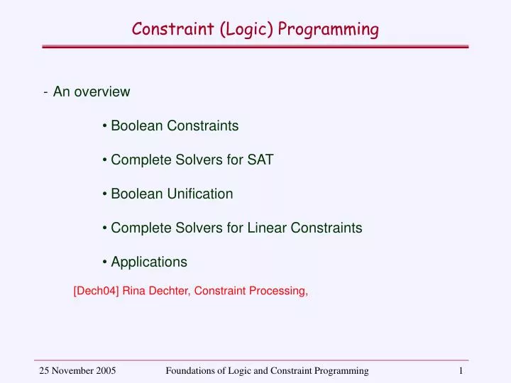
Constraint (Logic) Programming • An overview • Boolean Constraints • Complete Solvers for SAT • Boolean Unification • Complete Solvers for Linear Constraints • Applications [Dech04] Rina Dechter, Constraint Processing, Foundations of Logic and Constraint Programming
A C G1 S G2 B Boolean Constraints • Boolean domains (often referred to as 0/1 variables) has many applications, namely • In Digital Circuits • Exemple: Half-adder • In problems modelling binary choices • Exemple: N-Queens • In problems dealing with sets Foundations of Logic and Constraint Programming
Approaches to Boolean Constraint Solving • The satisfaction of Boolean constraints may be addresses in various and alternative ways • Simbolically • Boolean Unification • Complete Solver • SAT • All constraints are converted into Clauses (CNF) • Solution construction (backtracking) or repairing (local search) • Finite Domains • Booleans are just an instance of a Finite domain (0/1) • Techniques common to other Finite Domains Foundations of Logic and Constraint Programming
Boolean Constraints • To handle Boolean satisfaction simbolically, it is convenient to convert all Boolean constraints using exclusively equality constraint on Boolean Formulas. Boolean Formulas are composed of • Two Boolean operators # (exclusive or) and ·(conjunction), • Boolean constants 0 e 1 ( and possibly other constants, domain dependent) • variábles denoted by upper case letters • This conversion is always possible, since the set {0, 1, #, ·} is complete. Given arbitrary terms a and b, all the usual operators and constants may be expressed using exclusively the “#” and “·” operators. a= 1 # a ; ab = a ·b ; ab= a # b # a ·b ab= 1 # a # a ·b ; ab = 1 # a # b Foundations of Logic and Constraint Programming
Boolean Rings • More formally, the tuple < A, 0, 1, #, ·>, where A any domain that includes two elements 0 and 1, is a boolean ring, if the following properties are satisfied • Associativity a#(b#c) = (a#b)#c a·(b·c) = (a·b)·c • Comutativity a # b = b # a a · b = b · a • Distribution a #(b·c) = (a#b)·(a#c) a·(b#c) = a·b#a·c • Neutral Element a#0 = a a·1 = a • Exclusivity and Idempotence a#a = 0 a·a = a • Absorbing Element a·0 = 0 Foundations of Logic and Constraint Programming
Boolean Constraints on Sets • Although Boolean constraints are usually considered on domains with only two elements, another interesting domain of application is Sets. • More precisely, considering a domain P of all all sets composed of elements a1, a2, a3, ..., an • Constant 1 corresponds to the Universal set {a1, a2, a3, ..., an} • Constant 1 corresponds to the Empty set { } • Operator “#” corresponds to the Set Exclusive Union • Operator “·” corresponds to Set Intersection • Other constraints on setsmay be converted into equality. For example, given the equivalence ab ab= a ab= b the includes constraint ““can be rewritten as a # b # a·b = b a # b # b # a·b = b # b a # a·b = 0 a·b = a Foundations of Logic and Constraint Programming
Constraint Solving through Boolean Unification • The implementation of a symbolical and complete constraint solver fo Booleans is the core of CLP(B), the instance of the CLP(X) scheme to the Boolean Domain. • In this solver, Boolean constraints are maintained in a solved form, obtained through Boolean unification. • A Boolean constraint t1 = t2 (where terms t1 e t2are exclusively written has the form with operators “#” and “·” . Such constraint can be satisfied iff there is a Boolean Unifier for terms t1 and t2. • A Boolean unifier is a set of pairs x / t where x and t are respectively Boolean variables and terms (much in the same way of unifiers in logic programming), and where none of the variables may appear in the terms. • As in logic programming, Boolean unifiers will be denoted by greek letters. Foundations of Logic and Constraint Programming
Boolean Unification: Examples Example 1: Terms t1=1 # Aandt2 = A·B admit the following Boolean unifier = {A/1, B/0} In fact, denoting by t(or t) the application of substitution to term t, t1= (1#A){A/1, B/0}= 1 # 1 = 0 t2= (A·B){A/1, B/0}= 1 · 0 = 0 which guarantees that constraint t1 = t2 is satisfiable. Example 2: Terms t1 = 1 # A·B and t2= C # D admit unifiers a={C/1#A·B#D}andb = {C/1#D, A/0} since t1 a= (1#A·B){C/1#A·B#D} = 1#A·B t2 a= (C#D) {C/1#A·B#D} = 1#A·B#D#D = 1#A·B and t1 b= (1#A·B){C/1#D, A/0} = 1#0·B = 1 t2 b= (C#D) {C/1#D, A/0} = (1#D#D) = 1 Foundations of Logic and Constraint Programming
Multiple Boolean Unifiers • Like in LP it is convenient to consider a hierarchy of unifiers, related by the “more general” relationship. • Unifier a is more general then b : there is a substitution s such that b = a s. Example: As seen above, terms t1 = 1 # A·B and t2= C # D , admit unifiers a={C/1#A·B#D}andb = {C/1#D, A/0} In this case, a is more general than b, since for s = {A/0},it is b = a s. a s = {C/1#A·B#D } o {A / 0} = {C/1#D, A/0}= b Foundations of Logic and Constraint Programming
Most General Boolean Unifiers • In general, given two Boolean terms, t1 e t2, there might be not only more than one unifiers, but also more than one most general unifier. Example: Boolean terms t1 = 1 # A·B and t2= C # D may be unified by the most general unifiers 1 = { C / 1 # A·B # D} 2 = { D / 1 # A·B # C} 3 = { A / 1 # C # D, B / 1} 4 = { A / 1, B / 1 # C # D} • None of the unifiers may be obtained by the composition of any of the others and a substitution. Foundations of Logic and Constraint Programming
Boolean Unification Algorithm • Taking into account that constraint t1=t2 is equivalent to t1#t2= 0, the unification of terms t1 and t2is equivalent to constrain term t1#t2 to 0. The conditions necessary to zero a term t, may be analysed follows: • Zeroing a constant term is trivially checkable • If t = 0 the term is already zero; • If t = 1 term cannot be zeroed • Given distribution, a non constant term t, can always be written in the form a·U#b (where U is one of the variables occurring in t) factoring t in order to U. • A term t = a·U # b may onlty be zeroed if either a = 1 or b = 0, or both. Otherwise, i.e. a = 0 and b = 1, it would be t = 1 0, whatever the value chosen for U. 4. Such condition (a = 1 orb = 0) is guaranteed iff the term (1 # a)·b is zeroed. Foundations of Logic and Constraint Programming
Boolean Unification Algorithm • Once condition a = 1orb = 0 is guaranteed, • if a = 0 (and b = 0), then variable U may take an arbitraru value, since 0 = 0·U # 0) • if a = 1, then variable U must take valur b (in this case, 0 = 1·U # b) • The assignment to U of these terms can be implemented by means of a fresh variable, not occurring in t. Denoting by _U this new variable, the previous condition is equivalent to U = (1#a)·_U # b • In fact, • If a = 0 (and b = 0 ) then U = _U, i.e.U may take any arbitrary value, since variable _U, being a fresh variable, is not constrained anywhere. • If a = 1 then U = (1#1)·_U # b, i.e. U = b, as intendend. Foundations of Logic and Constraint Programming
Boolean Unification Procedure • The reasoning above can be used in the implementation of predicate unif_bool, shown below. predicate unif_bool(in: t1, t2; out: ); tt1 # t2; unif_bool zero(t,); end predicate. • The predicate inputs terms t1 and t2 , that are to be unified, and succeeds if predicate zero succeedes, returning unifier obtained from this predicate. Foundations of Logic and Constraint Programming
Boolean Unification Procedure Predicate zero can now be implemented as shpown below predicate zero (in: t; out: ); case t = 0: zero = True, = {}; case t = 1: zero = False; otherwise: A·u # B t; s (1#A)·B; if zero(s,σ) then zero True; {U/(1#A)·_U#B} o σ else zero = False end if end case end predicate Foundations of Logic and Constraint Programming
Boolean Unification Procedure: Example {U/(1#A)·_U#B} o σ • Notice that substitution b returned by predicate zero is obtained through the composition of substitutions {U/(1#A)·U#B} and σobtained from the recursive call of the predicate. Example: Satisfy constraint X # X·Z = Y·Z # 1 Unify X#X·Z and Y·Z#1 zero X#X·Z#Y·Z#1 = (1#Z)·X#Y·Z#1 % Ax·X#Bx zero (1#(1#Z))·(Y·Z#1) % (1#Ax)·Bx = Z·(Y·Z#1) = Z·Y#Z % Ay·Y#By zero (1#Z)·Z %(1#Ay)·By = 0 Foundations of Logic and Constraint Programming
Boolean Unification Algorithm: Example Now let us analyse the unifier that is returned by the sequence of calls Unify X#X·Z and Y·Z#1 zero X#X·Z#Y·Z#1 = (1#Z)·X#Y·Z#1 zero (1#(1#Z))·(Y·Z#1)=Z·Y#Z %(1#Ax)·Bx zero (1#Z)·Z = 0%(1#Ay)·By σz = {} σy = {Y/(1#Ay)·_Y#By} o σz = {Y/(1#Z) ·_Y#Z} o {} = {Y/(1#Z) ·_Y#Z} σx = {X/(1#Ax)·_Y#Bx} o σy = {X/(1#1#Z)·_X # Y·Z#1} o {Y/(1#Z)·_Y#Z} = {X/ Z·_X #Y·Z#1} o {Y/(1#Z)·_Y#Z} = {X/ Z·_X #((1#Z)·_Y#Z)·Z#1, Y/(1#Z)·_Y#Z} = {X/ Z·_X #Z#1, Y/(1#Z)·_Y#Z} = {X/ Z·_X #Z#1, Y/(1#Z)·_Y#Z} Foundations of Logic and Constraint Programming
Interpreting Unifiers • Hence, constraint X#X·Z = Y·Z#1is satisfiable, since the unification of terms X#X·ZandY·Z#1succeeds, returning the most general unifier = {X/Z·_X #Z#1, Y/(1#Z)·_Y#Z} • This result can be confirmed: (X#X·Z)= (Z·_X#Z#1)#(Z·_X#Z#1)·Z = (Z·_X#Z#1)#Z·_X = Z#1 (Y·Z#1) = ((1#Z)·_Y#Z)·Z#1) = Z#1 • Analysing the unifier we note that the two terms unify whenever • Z=0 and X = 1 and Y is arbitrary (Y =_Y) • Z=1 and Y = 1and X is arbitrary (X =_X) • The unifier has therefore the ground instances {X/1, Y/0, Z/0}, {X/1, Y/1, Z/0}, {X/0, Y/1, Z/1}, {X/1, Y/1, Z/1}. Foundations of Logic and Constraint Programming
A D R2 C F R1 R4 E R3 B Digital Circuits Application A simple example: • Model circuit below with Boolean constraints • How does the output relates (symbolically) with the inputs. • R1:Unifier 1is obtained by solving R1 C = 1 # A·B 1 ={C / 1 # A·B} • R2: Then 1is applied to R2 R2’: R2 1 :D = (1#A·C){C/1#A·B} D = (1#A·(1#A·B)) D = 1 # A # A·B R1: C = 1 # A·B R2: D = 1 # A·C R3: E = 1 # B·C R4: F = 1 # D·E Foundations of Logic and Constraint Programming
Digital Circuits Application • SolvingR2’: D = 1 # A # A·B unifier ’2 is obtained ’2= {D / 1 # A # A·B} • 2 is obtained by composition of 2’with 1 2= 1 o 2’ = {C/1#A·B} o {D/1#A#A·B} = {C/1#A·B, D/1#A#A·B} • R3: Applying2to R3, then R3’: R3 2 : E = (1#B·C){D/1#A#A·B, C/1#A·B} : E = 1#B·(1#A·B) : E = 1#B·(1#A·B) • SolvingR3’, unifier 3’is obtained 3’ = {E/1#B#A·B} • Now, 3’is composed with2 3= 2 o 3’ = {E/1#B#A·B} o {D/1#A#A·B} o {C/1#A·B} = {E/1#B#A·B, D/1#A#A·B, C/1#A·B} Foundations of Logic and Constraint Programming
Digital Circuits Application • R4: Finally, before solving R4, 3 is applied R4’: R43 : F = (1#D·E){E/1#B#A·B, D/1#A#A·B, C/1#A·B} : F = 1#(1#A#A·B)·(1#B#A·B) : F = 1#1#B#A·B#A#A·B#A·B#A·B#A·B#A·B : F = A # B • Now, R4’is solved and unifier 4’ is obtained 4’ = {F/A#B} • Composing4’with 3, it is obtained 4, a unifier for all the constraints 4= 3 o 4’ = {E/1#B#A·B, D/1#A#A·B, C/1#A·B}o{F/A#B} = {E/1#B#A·B, D/1#A#A·B, C/1#A·B, F/A#B} • By interpreting 4 we may conclude that this circuit with 4 nand gates implements the exclusive-or, since F / A # B. Foundations of Logic and Constraint Programming
CLP(B) in SICStus • Once loaded SICStus Prolog the module on Boolean Constraints is loaded with directive :- use_module(library(clpb)). • Boolean Constraints may be specified with built-in predicate sat(E) , where equality is specified as ‘=:=’ and several Boolean operators can be used, namely C = or(A,B) specified as C =:= A+B C = nor(A,B) specified as C =\= A+B C = xor(A,B) specified as C =\= A#B C = and(A,B) specified as C =:= A*B C = nand(A,B) specified as C =\= A*B C = not(A) specified as C =\= A Foundations of Logic and Constraint Programming
CLP(B) in SICStus Some Examples: 1. ?- sat(A#B=:=F). sat(A =:= B#F)? % Constraint A#B = F is satisfiable with unifier A / B+F 2. ?- sat(A*B=:=1#C*D).sat(A=\=C*D#B)? % Constraint A·B=1+C·D is satisfiable with unifier A/1+C·D+B 3. ?- sat(A#B=:=1#C*D), sat(C#D=:=B). sat(B=:=C#D), sat(A=\=C*D#C#D) ? % Constraints A+B=1+C·D and B=C+D are satisfiable with unifier {A/1+C·D+C+D, B/C+D} Foundations of Logic and Constraint Programming
A D G2 C F G1 G4 E G3 B CLP(B) in SICStus :- use_module(library(clpb)). nand_gate(X,Y,Z):- sat(X*Y =:= 1#Z). circuit(A,B,[C,D,E],F):- nand_gate(A,B,C), nand_gate(A,C,D), nand_gate(B,C,E), nand_gate(D,E,F). A more complete example, related to the previous circuit | ?- circuit(A,B,[C,D,E],1). C = 1, E = A, sat(B=\=A), sat(D=\=A) ? Note: Compare this answer with unifier5 = {E/1+B, D/B, C/1, F/1, A/1+B } found before. Foundations of Logic and Constraint Programming
CLP(Q) Application • Another domain for which a complete solver exists is that of linear constraints over the rationals or reals. The integration of such a solver with LP forms the CLP(Q) or CLP(R) instance of the CLP(X) scheme. • CLP(Q) and CLP(R) differ in their approach handle arithmetics: • If the coeficients are rational (division between integers) the solutiona are also rational. Hence CLP(Q) avoids rounding errors by handling properly with arithmetics (“+”,” –”, “*”, “/”) over rationals (with arithmetics without rounding • CLP(R) rounds rationals as floating point numbers, and is more “efficient” if less “precise” • These constraints are quite common in applications. Even when constraints are not linear, problems are often “linearised” (i.e. modelled with linear constraints such taht the errors are acceptable), given the very efficient way of solving these constraints, based on the SIMPLEX algorithm. Foundations of Logic and Constraint Programming
x 7 5/a 3/b y 9 9 8/e 2/d 7/c 13 8 z 6/f CLP(Q) : Example • The following problem illustrates a typical use of linear constraints: • Problem (Network Management): • Find the value of traffic from points x,y to z such that the traffic does not exceed the flow capacity of each arc, nor the processing capacity of each node. Contraints: % Minimum required flow x 6, z 10 % minimum flow % flow capacity of arcs a 5, b 3, c 7, d 2, e 8, f 6 % processing capacity of nodes x 7, y 9, a + b 9, c 8, a + b + d 9, e + f 13 % flow maintenance x = a, y = b + c, a + b + d = e, c = d + f, e + f = z % non-negative constraints x, y ,z, a, b, c, d, e, f 0 Foundations of Logic and Constraint Programming
CLP(Q) Solver: SIMPLEX • The SIMPLEX algorithm aims at converting all linear constraints into a solved form, composed of equality constraints on linear expressions. This conversion is done in two steps. • All inequality constraints on decision variables are converted into equality constraints with the addition of “slack” (non-negative) variables a X1 +...+ an Xn ≤ b a X1 +...+ an Xn + S = b a X1 +...+ an Xn ≥ b a X1 +...+ an Xn - S = b • In general m constraints on n decision variables are converted into m constraints on k+n non-negative variables, where k m ( k = m if all constraints are inequality constraints). • A solved form is obtained if a partition can be found on the k+n variables in m basic variables Xi (i 1..n) and p = k+n-m non basic variables Yj (j 1.. p), such that the m constraints can be written as Xi = di + ci1 Y1+ ... + cip Yp( for all i 1..n) where all free coefficients di are non-negative. Foundations of Logic and Constraint Programming
X2 x1 = 1 - x3/3 + x5/3 x2 = 6 - x3/3 - 2 x5/3 x4 = 4 - 2 x3/3 - X5/3 X2 = 5 + X1 - X5 X3 = 3 - 3 X1 + X5 X4 = 2 + 2 X1 - X5 2X1 + X2 ≤ 8 X1 + X2 ≥ 3 X1 - X2 ≥ -5 X1 , X2 ≥ 0 X5 = 0 X1 =0 X3 = 0 2X1 + X2 + X3 =8 X1 + X2 - X4 = 3 X1 - X2 - X5 =-5 X4 = 0 X1 X2 =0 X1 = 5 - X3 - X4 X2 = -2 + X3 + 2X4 X5 = 12 - 2 X3 - 3 X4 X3 =8- 2 X1 - X2 X4 = -3 + X1 + X2 X5 = 5+ X1 - X2 SIMPLEX: Geometric Interpretation Foundations of Logic and Constraint Programming
SICStus CLP(Q)/CLP(R) Solvers • SICStus Prolog supports constraint solving over the Rational/Real numbers. As for Booleans, to handle these constraints, a module for CLP(Q) or CLP(R) must be loaded, with directives: :- use_module(user:library(clpq)). :- use_module(user:library(clpr)). • Contraints may now be specified with the usual Prolog syntax but inside { }. For example the previous problem may be directly specified as p1([X1,X2]) :- {2*X1 + X2 =< 8, X1 + X2 >= 3, X1 - X2 >= -5 }, { X1 >= 0, X2 >= 0 }. or specified with explicit slack variables p2([X1,X2,X3,X4,X5]) :- {2*X1+X2+X3 = 8, X1+X2–X4 = 3, X1-X2–X5 = -5 }, { X1 >= 0, X2 >= 0, X3 >= 0, X4 >= 0, X5 >= 0} . Foundations of Logic and Constraint Programming
X2 X1 -X2 =-5 X1 >=0 2 X1 + X2 = 8 X1 +X2 =3 X1 X2 >=0 SICStus CLP(Q)/CLP(R) Solvers • Once defined these programs can be run. Answers projected to the called variables, with some extra variables included when necessary p1([X1,X2]) :- {2*X1 + X2 =< 8, X1 + X2 >= 3, X1 - X2 >= -5 }, { X1 >= 0, X2 >= 0 }. | ?- p1([X1,X2]). {X1+1/2*X2=<4}, {X1>=0}, {X2>=0}, {X1+X2>=3}, {X1-X2>= -5} ? Foundations of Logic and Constraint Programming
X2 X1 -X2 =-5 X1 >=0 2 X1 + X2 = 8 X1 +X2 =3 X1 X2 >=0 SICStus CLP(Q)/CLP(R) Solvers • The solved form is more easily (?) identified with the explicit slack variables. p2([X1,X2,X3,X4,X5]) :- {2*X1+X2+X3 = 8, X1+X2–X4 = 3, X1-X2–X5 = -5 }, { X1 >= 0, X2 >= 0, X3 >= 0, X4 >= 0, X5 >= 0} . | ?- p2([X1,X2,X3,X4,X5]). {X5=9-3/2*X2-1/2*X3}, {X4=1+1/2*X2-1/2*X3}, {X1=4-1/2*X2-1/2*X3}, {X2+X3=<8}, {X2+1/3*X3=<6}, {X2>=0}, {X3>=0}, {X2-X3>= -2} ? • Solved form identifies X1 = 4, X2 = 0 Foundations of Logic and Constraint Programming
X2 X1 -X2 =-5 X1 >=0 2 X1 + X2 = 8 X1 +X2 =3 X1 X2 >=0 SICStus CLP(Q)/CLP(R) Solvers • Of course, if the problem has no solutions the answer is no! p3([X1,X2]) :- {2*X1 + X2 >= 8, X1 + X2 =<3, X1-X2=<-5 }, { X1 >= 0, X2 >= 0} . | ?- p3([X1,X2]). no ? Foundations of Logic and Constraint Programming
SICStus CLP(Q)/CLP(R): Example Example: A certain amount of money is lent at some interest rate for a number of time periods, to be payed with constant instalments. Model Assuming that • I is the number of time periods remaining to pay the debt • Di represents the debt at the begining of time period i. • R is the interest rate (in percentage points) • P is the (constant) instalment to be payed at the end of each time period then we have the following relations: • The debt at the begining of a period is the debt at the begining of the previous period, increased by the interest, less the payment made. Di = Di+1 * (1 +R/100) – P for i > 1 • No debt should exist at the end of the last time period last time period 0 = D1 * (1 +R/100) – P Foundations of Logic and Constraint Programming
SICStus CLP(Q)/CLP(R): Example • These constraints can be easily expressed in CLP(Q) / CLP(R) as shown in the programs below. • Notice that such program could not be easily converted to pure Prolog, in statements like V is Exp, since one does not know what values are given and what are know. % 0 = D1 * (1 +R/100) – P debt(Debt, Rate, TimeLeft, Payment):- { TimeLeft = 1, Payment = Debt * (1 + Rate/100) }. % Di = Di+1 * (1 +R/100) – P for i > 1 debt(Debt, Rate, TimeLeft, Payment):- { TimeLeft > 1, NextTimeLeft = TimeLeft - 1, NextDebt = Debt * (1 + Rate/100) – Payment }, debt(NextDebt, Rate, NextTimeLeft, Payment). Foundations of Logic and Constraint Programming
SICStus CLP(Q)/CLP(R): Example Some interaction with the program • What yearly payment is due when 100 units are lent for 7 years at a 5% interest rate. What is the total payment? | ?-debt(100,5,7,P), {T = 7* P}. P = 17.28198184461708, T = 120.97387291231955 ? • What amount of money can be borrowed by someone that is willing to pay a fixed instalment of 10 units for 7 years, whne the interest rate is 5%? | ?-debt(D,5,7,10). D = 57.86373397397567 ? • What is the relationship between the yearly payment and the initial debt, when 7 years are used and the interest rate is 5%? | ?-debt(D,5,7,P). {P=0.17281981844617078*D} ? Foundations of Logic and Constraint Programming
SICStus CLP(Q)/CLP(R): Example • It is important to notice that CLP(Q)/CLP(R) is only complete when the constraints are linear. When they are not they are frozen in the constraint store, pending further instantiation • What is the relation between the yearly payment and the initial debt, when 7 years are used and the interest rate is R% | ?-debt(D,R,7,10). clpr:{10.0-D-0.01*(R*D)+_A=0.0}, % 7 years to go clpr:{10.0-0.01*(_B*R)-_B=0.0}, % 6 years to go clpr:{10.0+_C-0.01*(_A*R)-_A=0.0}, % 5 years to go clpr:{10.0+_D-0.01*(_C*R)-_C=0.0}, % 4 years to go clpr:{10.0+_E-0.01*(_D*R)-_D=0.0}, % 3 years to go clpr:{10.0+_F-0.01*(_E*R)-_E=0.0}, % 2 years to go clpr:{10.0+_B-0.01*(_F*R)-_F=0.0} ?% 1 years to go Foundations of Logic and Constraint Programming