Download
1 / 47
470 likes | 552 Views
One of these will be true… but you don’t know which one. You’ll make one of these claims, based on your observations. Why are we even HERE?. Unbiased Estimators are statistics which accurately target the parameters they aim to target (catch them “on average”). . In the interest of time…

E N D
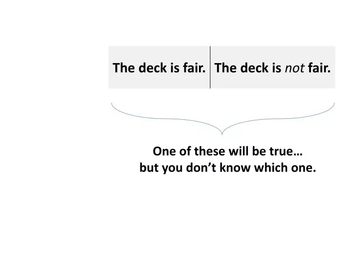
One of these will be true… but you don’t know which one.
You’ll make one of these claims, based on your observations
Unbiased Estimatorsarestatistics which accurately target the parameters they aim to target (catch them “on average”).
In the interest of time… (10 weeks time I would like to have)
Each individual statistic will most likely be “off” a bit in value from the parameter (“sampling error”)…for example…
…so, in MTH 244, we will learn to build “wings” around our statistics to mitigate as much error as possible…
To properly estimate a parameter from a sample, you need to form a confidence interval (CI)… • (remember 2?)
The Wonderful Binomial Distribution! (fixed number of trials n, constant probability of success p) Sampling Based on the W.B.D.! (population believed to have constant, but unknown, probability of success p)
(January, 2010) A random sample of 702 “for sale” Bend single – family homes (FSBSFH) showed 65 were in foreclosure. What percentage of all Bend “for sale” homes were in foreclosure in January 2010 (at 95% confidence)? (April, 2013) A random sample of 1734 FSBSFH homes shows that 163 are in foreclosure. What percentage of all Bend “for sale” homes were in foreclosure in April 2013 (again, at 95% confidence)? How does it compare to 1.2010? (December, 2013) A newer random sample of FSBSFH 81 out of a sample of 1102 are in foreclosure. What percentage of all Bend “for sale” homes were in foreclosure in December 2013 (again, at 95% confidence)? How does it compare to the previous ones? (December, 2013) Looks like there are 20,533 SFH for sale in Oregon as I type this (not a sample!). Of them, 1992 are in foreclosure. How does the State of Oregon’s overall foreclosure rate compare to Bend’s? Any MMD’s? “Statistics require MOE’s – Parameters stand alone.”
You might recall (from MTH 243) that binomial distributions’ histograms begin to look like bell curves if 1) p 0.5 and 2) n is very large.
You might recall (from MTH 243) that binomial distributions’ histograms begin to look like bell curves if 1) p 0.5 and 2) n is very large.
You might recall (from MTH 243) that binomial distributions’ histograms begin to look like bell curves if 1) p 0.5 and 2) n is very large.
You might recall (from MTH 243) that binomial distributions’ histograms begin to look like bell curves if 1) p 0.5 and 2) n is very large.
You might recall (from MTH 243) that binomial distributions’ histograms begin to look like bell curves if 1) p 0.5 and 2) n is very large.
You might recall (from MTH 243) that binomial distributions’ histograms begin to look like bell curves if 1) p 0.5 and 2) n is very large.
So, for a given value of p (close to 0.5), as n , the distribution resembles a normal distribution more and more. But, what if p varies? In the next few slides, n = 20.
So, as p begins to vary significantly from 0.5, the distributions skew more and more. But…watch what happens when n , even when p = 0.1 (highly skewed)...
n= 20 np= 20(0.1) = 2
n= 40 np= 40(0.1) = 4
n= 60 np= 60(0.1) = 6
n= 80 np= 80(0.1) = 8
n= 100 np= 100(0.1) = 10
So long as we can ensure that our sample is big enough (that is, np 5 and nq 5), our methods of proportional CI’s will be valid. It’s an even better fit when np 10 and nq 10. • (For a formal proof, check the enrichment page of the website)