Download
1 / 63
630 likes | 633 Views
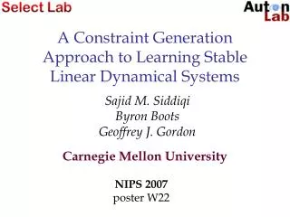
This research explores a constraint generation approach to learning stable linear dynamical systems for dynamic textures. It focuses on videos of moving scenes with stationary properties, aiming to capture their dynamics through low-dimensional models. The learned models can be used for applications such as compression, recognition, and synthesis of videos.

E N D
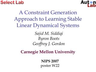
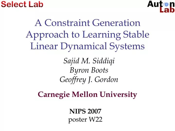
A Constraint Generation Approach to Learning Stable Linear Dynamical Systems Sajid M. SiddiqiByron BootsGeoffrey J. Gordon Carnegie Mellon University NIPS 2007poster W22
Application: Dynamic Textures1 • Videos of moving scenes that exhibit stationarity properties • Dynamics can be captured by a low-dimensional model • Learned models can efficiently simulate realistic sequences • Applications: compression, recognition, synthesis of videos steam river fountain 1 S. Soatto, D. Doretto and Y. Wu. Dynamic Textures. Proceedings of the ICCV, 2001
Linear Dynamical Systems • Input data sequence
Linear Dynamical Systems • Input data sequence
Linear Dynamical Systems • Input data sequence • Assume a latent variable that explains the data
Linear Dynamical Systems • Input data sequence • Assume a latent variable that explains the data
Linear Dynamical Systems • Input data sequence • Assume a latent variable that explains the data • Assume a Markov model on the latent variable
Linear Dynamical Systems • Input data sequence • Assume a latent variable that explains the data • Assume a Markov model on the latent variable
Linear Dynamical Systems2 • State and observation models: • Dynamics matrix: • Observation matrix: 2 Kalman, R. E. (1960). A new approach to linear filtering and prediction problems. Trans.ASME-JBE
Linear Dynamical Systems2 • State and observation models: • Dynamics matrix: • Observation matrix: • This talk: • Learning LDS parameters from data while ensuring a stable dynamics matrix Amore efficiently and accurately than previous methods 2 Kalman, R. E. (1960). A new approach to linear filtering and prediction problems. Trans.ASME-JBE
Learning Linear Dynamical Systems • Suppose we have an estimated state sequence
Learning Linear Dynamical Systems • Suppose we have an estimated state sequence • Define state reconstruction error as the objective:
Learning Linear Dynamical Systems • Suppose we have an estimated state sequence • Define state reconstruction error as the objective: • We would like to learn such that i.e.
Subspace Identification3 • Subspace ID uses matrix decomposition to estimate the state sequence 3 P.Van Overschee and B. De Moor Subspace Identification for Linear Systems. Kluwer, 1996
Subspace Identification3 • Subspace ID uses matrix decomposition to estimate the state sequence • Build a Hankel matrixD of stacked observations 3 P.Van Overschee and B. De Moor Subspace Identification for Linear Systems. Kluwer, 1996
Subspace Identification3 • Subspace ID uses matrix decomposition to estimate the state sequence • Build a Hankel matrixD of stacked observations 3 P.Van Overschee and B. De Moor Subspace Identification for Linear Systems. Kluwer, 1996
Subspace Identification3 • In expectation, the Hankel matrix is inherently low-rank! 3 P.Van Overschee and B. De Moor Subspace Identification for Linear Systems. Kluwer, 1996
Subspace Identification3 • In expectation, the Hankel matrix is inherently low-rank! 3 P.Van Overschee and B. De Moor Subspace Identification for Linear Systems. Kluwer, 1996
Subspace Identification3 • In expectation, the Hankel matrix is inherently low-rank! 3 P.Van Overschee and B. De Moor Subspace Identification for Linear Systems. Kluwer, 1996
Subspace Identification3 • In expectation, the Hankel matrix is inherently low-rank! • Can use SVD to obtain the low-dimensional state sequence 3 P.Van Overschee and B. De Moor Subspace Identification for Linear Systems. Kluwer, 1996
Subspace Identification3 • In expectation, the Hankel matrix is inherently low-rank! • Can use SVD to obtain the low-dimensional state sequence For D with k observations per column, = 3 P.Van Overschee and B. De Moor Subspace Identification for Linear Systems. Kluwer, 1996
Subspace Identification3 • In expectation, the Hankel matrix is inherently low-rank! • Can use SVD to obtain the low-dimensional state sequence For D with k observations per column, = 3 P.Van Overschee and B. De Moor Subspace Identification for Linear Systems. Kluwer, 1996
Lets train an LDS for steam textures using this algorithm, and simulate a video from it! = [ …] xt2 R40
Simulating from a learned model xt t The model is unstable
Notation • 1 , … , n : eigenvalues of A (|1| > … > |n| ) • 1,…,n: unit-length eigenvectors of A • 1,…,n: singular values of A (1 > 2 > … n) • S : matrices with |1| · 1 • S : matrices with1 · 1
Stability • a matrix A is stable if |1|· 1, i.e. if
Stability • a matrix A is stable if |1|· 1, i.e. if
Stability • a matrix A is stable if |1|· 1, i.e. if |1| = 0.3 |1| = 1.295
Stability • a matrix A is stable if |1|· 1, i.e. if xt(1), xt(2) |1| = 0.3 xt(1), xt(2) |1| = 1.295
Stability • a matrix A is stable if |1|· 1, i.e. if • We would like to solve xt(1), xt(2) |1| = 0.3 xt(1), xt(2) |1| = 1.295 s.t.
Stability and Convexity • ButS is non-convex!
Stability and Convexity • ButS is non-convex! A1 A2
Stability and Convexity • ButS is non-convex! • Lets look at S instead … • S is convex • S µS A1 A2
Stability and Convexity • ButS is non-convex! • Lets look at S instead … • S is convex • S µS A1 A2
Stability and Convexity • ButS is non-convex! • Lets look at S instead … • S is convex • S µS • Previous work4exploits these properties to learn a stable A bysolving the semi-definite program A1 A2 s.t. 4 S. L. Lacy and D. S. Bernstein. Subspace identification with guaranteed stability using constrained optimization. In Proc. of the ACC (2002), IEEE Trans. Automatic Control (2003)
Lets train an LDS for steam again, this time constraining A to be in S
Simulating from a Lacy-Bernstein stable texture model xt t Model is over-constrained.Can we do better?
Our Approach • Formulate the S approximation of the problem as a semi-definite program (SDP) • Start with a quadratic program (QP)relaxation of this SDP, and incrementally add constraints • Because the SDP is an inner approximation of the problem, we reach stabilityearly, before reaching the feasible set of the SDP • We interpolate the solution to return the best stable matrix possible
The Algorithm objective function contours
The Algorithm objective function contours • A1: unconstrained QP solution (least squares estimate)
The Algorithm objective function contours • A1: unconstrained QP solution (least squares estimate)
The Algorithm objective function contours • A1: unconstrained QP solution (least squares estimate) • A2:QP solution after 1 constraint (happens to be stable)
The Algorithm objective function contours • A1: unconstrained QP solution (least squares estimate) • A2:QP solution after 1 constraint (happens to be stable) • Afinal:Interpolation of stable solution with the last one
The Algorithm objective function contours • A1: unconstrained QP solution (least squares estimate) • A2:QP solution after 1 constraint (happens to be stable) • Afinal:Interpolation of stable solution with the last one • Aprevious method:Lacy Bernstein (2002)
Lets train an LDS for steam using constraint generation, and simulate …
Simulating from a Constraint Generation stable texture model xt t Model captures more dynamics and is still stable
Least Squares • Constraint Generation
Empirical Evaluation • Algorithms: • Constraint Generation – CG (our method) • Lacy and Bernstein (2002) –LB-1 • finds a 1· 1 solution • Lacy and Bernstein (2003)–LB-2 • solves a similar problem in a transformed space • Data sets • Dynamic textures • Biosurveillance baseline models (see paper)