Understanding the TSL EBSD Data Collection System

1. Understanding the TSL EBSD Data Collection System Harry Chien, Bassem El-Dasher, Anthony Rollett, Gregory Rohrer

2. Overview • Understanding the diffraction patterns • Source of diffraction • SEM setup per required data • The makeup of a pattern • Setting up the data collection system • Environment variables • Phase and reflectors • Capturing patterns • Choosing video settings • Background subtraction • Image Processing • Detecting bands: Hough transform • Enhancing the transform: Butterfly mask • Selecting appropriate Hough settings • Origin of Image Quality (I.Q.)

3. Overview (cont’d) • Indexing captured patterns • Identifying detected bands: Triplet method • Determining solution: Voting scheme • Origin of Confidence Index (C.I.) • Identifying a solution in multi-phase materials • Calibration • Physical meaning • Method and need for tuning • Scanning • Choosing appropriate parameters

4. SEM Schematic Overview • All students using this system need to know how to use SEM. It is recommended that all users take SEM courses offered by the MSE department

5. Sample Size effect • All the samples needs to be prepared (polished) before EBSD data collection. As most samples are mounted before polishing, it is recommended to use smaller size mount (1.25 inch preferred) • It is difficult to work with large mounted samples (with 1.5 inch) in OIM as the edge of the mount may touch either the camera or the SEM emitter after tilting • It is critically important that the specimen does NOT touch the phosphor screen because this is easily damaged 1.5 inch 1.25 inch

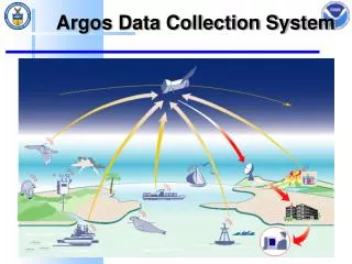
6. Diffraction Pattern-Observation Events • OIM computer asks Microscope Control Computer to place a fixed electron beam on a spot on the sample • A cone of diffracted electrons is intercepted by a specifically placed phosphor screen • Incident electrons excite the phosphor, producing photons • A Charge Coupled Device (CCD) Camera detects and amplifies the photons and sends the signal to the OIM computer for indexing

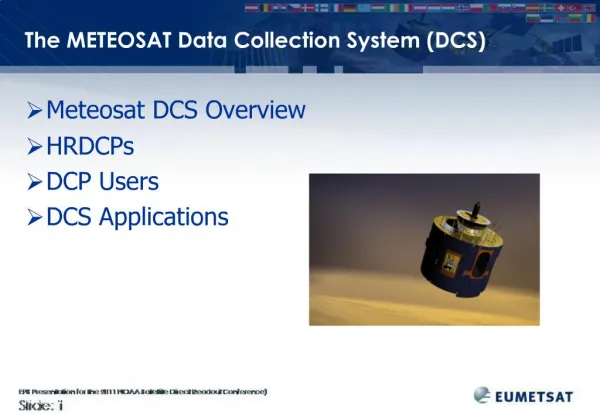
7. Vacuum System • The Quanta FEG has 3 operating vacuum modes to deal with different sample types: • High Vacuum • Low Vacuum • ESEM (Environmental SEM) • Low Vacuum and ESEM can use water vapours from a built-in water reservoir which is supplied by the user and connected to a gas inlet provided. • Observation of outgassing or highly charging materials can be made using one of these modes without the need to metal coat the sample.

8. Vacuum Status • Green: PUMPED to the desired vacuum mode • Orange: TRANSITION between two vacuum modes (pumping / venting / purging) • Grey: VENTED for sample or detector exchange

9. The Tool Bar Surface Positioning detector (automatically detect working Distance) Image Refreshing rate Turtle: lower refresh rate Rabbit: Higher refresh rate (higher resolution) Automatic Contrast and Brightness (short key F9)

10. Eucentric Position Note that eucentric position only occurs when the working distance is 10.

11. Diffraction Patterns-Source • Electron Backscatter Diffraction Patterns (EBSPs) are observed when a fixed, focused electron beam is positioned on a tilted specimen • Tilting is used to reduce the path length of the backscattered electrons • To obtain sufficient backscattered electrons, the specimen is tilted between 55-75o, where 70o is considered ideal • The backscattered electrons escape from 30-40 nm underneath the surface, hence there is a diffracting volume • Note that and 20-35o e- beam dz dy dx

12. X X X X Diffraction Patterns-Anatomy of a Pattern • There are two distinct features: • Bands • Poles Bands are intersections of diffraction cones that correspond to a family of crystallographic planes • Band widths are proportional to the inverse interplanar spacing • Intersection of multiple bands (planes) correspond to a pole of those planes (vector) • Note that while the bands are bright, they are surrounded by thin dark lines on either side

13. Diffraction Pattern-SEM Settings • Increasing the Accelerating Voltage increases the energy of the electrons Increases the diffraction pattern intensity • Higher Accelerating Voltage also produces narrower diffraction bands (a vs. b) and is necessary for adequate diffraction from coated samples (c vs. d) • Larger spot sizes (beam current) may be used to increase diffraction pattern intensity • High resolution datasets and non-conductive materials require lower voltage and spot size settings

14. System setup-Material data • In order for the system to index diffraction patterns, three material characteristics need to be known: • Symmetry • Lattice parameters • Reflectors • Information for most materials exist in TSL .mat files • “Custom” material files can be generated using the ICDD powder diffraction data files • Symmetry and Lattice parameters can be readily input from the ICDD data • Reflectors with the highest intensity should be used (4-5 reflectors for high symmetry; up to 12 reflectors for low symmetry)

15. System setup-Material data • Enter appropriate material parameters • Reflectors should be chosen based on: • Intensity • The number per zone

16. Pattern capture-Background Live signal Averaged signal • The background is the fixed variation in the captured frames due to the spatial variation in intensity of the backscattered electrons • Removal is done by averaging 8 frames (SEM in TV scan mode) • Note the variation of intensity in the images. The brightest point (marked with X) should be close to the center of the captured circle. • The location of this bright spot can be used to indicate how appropriate the Working Distance is. A low bright spot = WD is too large and vice versa

17. Pattern capture-Background Subtraction Without subtraction With subtraction • The background subtraction step is critical as it “brings out” the bands in the pattern • The “Balance” slider can be used to aid band detection. Usually a slightly lower setting improves indexing even though it may not appear better to the human eye

18. Detecting Patterns-The Hough of one band Cartesian space Transformed (Hough) space • Since the patterns are composed of bands, and not lines, the observed peaks in Hough space are a collection of points and not just one discrete point • Lines that intersect the band in Cartesian space are on average higher than those that do not intersect the band at all

19. Setting up binning/mask • Due to the shape of a band in Hough space, a multiplicative mask can be used to intensify the band grayscale • Three mask sizes are available: 5 x 5, 9 x 9, 13 x 13. These numbers refer to the pixel size of the mask • A 5 x 5 block of pixels is processed at a time • The grayscale value of each pixel is multiplied by the corresponding mask value • The total value is added to the grayscale value at the center of the mask • Note that the sum of the mask elements = zero 5 x 5 mask

20. Detecting Patterns-Hough Parameters Symmetry 0 Symmetry 1 Binned Pattern Size=Hough resolution in r I.Q.=Average grayscale value of detected Hough peaks

21. Indexing Patterns-Identifying Bands • Procedure: • Generate a lookup table from given lattice parameters and chosen reflectors (planes) that contains the inter-planar angles • Generate a list of all triplets (sets of three bands) from the detected bands in Hough space • Calculate the inter-planar angles for each triplet set • Since there is often more than one possible solution for each triplet, a method that uses all the bands needs to be implemented

22. Indexing Patterns-Settings Tolerance = How much angular deviation a plane is allowed while being a candidate Band widths: check if the theoretical width of bands should be considered during indexing If multi-phase indexing is being used, a “best” solution for each phase will be calculated. These values assign a weight to each possible factor: • Votes: based on total votes for the solution/largest number of votes for all phases • CI: ratio of CI/largest CI for all phases • Fit: fit for the solution/best (smallest) fit between all phases The indexing solution of the phase with the largest Rank value is chosen as the solution for the pattern

23. Solution # Band triplets # votes Indexing Patterns-Voting Scheme • Consider an example where there exist: • Only 10 band triplets (i.e. 5 detected bands) • Many possible solutions to consider, where each possible solution assigns an hkl to each band. Only 11 solutions are shown for illustration • Triplets are illustrated as 3 colored lines • If a solution yields inter-planar angles within tolerance, a vote or an “x” is marked in the solution column • The solution chosen is that with most number of votes • Confidence index (CI) is calculated as • Once the solution is chosen, it is compared to the Hough and the angular deviation is calculated as the fit S1 (solution w/most votes) S2 (solution w/ 2ndmost votes)

24. Scanning • The selection of scanning parameters depends on some factors: • Time allotted • Desired area of coverage (scan size) • Desired detail (step size) • To determine if the scan settings are acceptable time-wise you must: • Start the scan • Use a watch and note how many patterns are solved per minute (n) • Divide the total number of points by n to get the total time • To decide if the step size is appropriate for your SEM settings, use the following rough guide: