Download
1 / 90
1.5k likes | 2.75k Views
Chapter 2 Optical Resonator and Gaussian Beam optics. What is an optical resonator?.

E N D
What is an optical resonator? An optical resonator, the optical counterpart of an electronic resonant circuit, confines and stores light at certain resonance frequencies. It may be viewed as an optical transmission system incorporating feedback; light circulates or is repeatedly reflected within the system, without escaping. Chapter 2 Optical resonator and Gaussian beam
Contents • 2.1 Matrix optics • 2.2 Planar Mirror Resonators • Resonator Modes • The Resonator as a Spectrum Analyzer • Two- and Three-Dimensional Resonators • 2.3 Gaussian waves and its characteristics • The Gaussian beam • Transmission through optical components • 2.4 Spherical-Mirror Resonators • Ray confinement • Gaussian Modes • Resonance Frequencies • Hermite-Gaussian Modes • Finite Apertures and Diffraction Loss Chapter 2 Optical resonator and Gaussian beam
2.1 Brief review of Matrix optics Light propagation in a optical system, can use a matrix M, whose elements are A, B, C, D, characterizes the optical system Completely ( known as the ray-transfer matrix.) to describe the rays transmission in the optical components. One can use two parameters: y: the high q: the angle above z axis Chapter 2 Optical resonator and Gaussian beam
d y2 y1 For the paraxial rays y2,q2 -q2 y1,q1 q1 q Along z upward angle is positive, and downward is negative Chapter 2 Optical resonator and Gaussian beam
Free-Space Propagation Refraction at a Planar Boundary Refraction at a Spherical Boundary Transmission Through a Thin Lens Reflection from a Spherical Mirror Reflection from a Planar Mirror Chapter 2 Optical resonator and Gaussian beam
A Set of Parallel Transparent Plates. Matrices of Cascaded Optical Components Chapter 2 Optical resonator and Gaussian beam
Periodic Optical Systems The reflection of light between two parallel mirrors forming an optical resonator is a periodic optical system is a cascade of identical unit system. Difference Equation for the Ray Position A periodic system is composed of a cascade of identical unit systems (stages), each with a ray-transfer matrix (A, B, C, D). A ray enters the system with initial position y0 and slope 0. To determine the position and slope (ym,m) of the ray at the exit of the mth stage, we apply the ABCD matrix m times, Chapter 2 Optical resonator and Gaussian beam
From these equation, we have So that And then: linear differential equations, where and Chapter 2 Optical resonator and Gaussian beam
If we assumed: So that, we have If we defined We have then A general solution may be constructed from the two solutions with positive and negative signs by forming their linear combination. The sum of the two exponential functions can always be written as a harmonic (circular) function, Chapter 2 Optical resonator and Gaussian beam
If F=1, then Condition for a Harmonic Trajectory: if ym be harmonic, the f=cos-1b must be real, We have condition or The bound therefore provides a condition of stability (boundedness) of the ray trajectory If, instead, |b| > 1, f is then imaginary and the solution is a hyperbolic function (cosh or sinh), which increases without bound. A harmonic solution ensures that y, is bounded for all m, with a maximum value of ymax. The bound |b|< 1 therefore provides a condition of stability (boundedness) of the ray trajectory. Chapter 2 Optical resonator and Gaussian beam
Condition for a Periodic Trajectory Unstable b>1 Stable and periodic Stable nonperiodic The harmonic function is periodic in m, if it is possible to find an integer s such that ym+s = ym, for all m. The smallest such integer is the period. The necessary and sufficient condition for a periodic trajectory is: sf = 2pq, where q is an integer Chapter 2 Optical resonator and Gaussian beam
EXERCISE A Periodic Set of Pairs of Different Lenses. Examine the trajectories of paraxial rays through a periodic system composed of a set of lenses with alternating focal lengths f1 and f2 as shown in Fig. Show that the ray trajectory is bounded (stable) if Chapter 2 Optical resonator and Gaussian beam
Home work • Ray-Transfer Matrix of a Lens System. Determine the ray-transfer matrix for an optical system made of a thin convex lens of focal length f and a thin concave lens of focal length -f separated by a distance f. Discuss the imaging properties of this composite lens. Chapter 2 Optical resonator and Gaussian beam
Home works 2. 4 X 4 Ray-Transfer Matrix for Skewed Rays. Matrix methods may be generalized to describe skewed paraxial rays in circularly symmetric systems, and to astigmatic (non-circularly symmetric) systems. A ray crossing the plane z = 0 is generally characterized by four variables-the coordinates (x, y) of its position in the plane, and the angles (e,, ey) that its projections in the x-z and y-z planes make with the z axis. The emerging ray is also characterized by four variables linearly related to the initial four variables. The optical system may then be characterized completely, within the paraxial approximation, by a 4 X 4 matrix. (a) Determine the 4 x 4 ray-transfer matrix of a distance d in free space. (b) Determine the 4 X 4 ray-transfer matrix of a thin cylindrical lens with focal length f oriented in the y direction. The cylindrical lens has focal length f for rays in the y-z plane, and no focusing power for rays in the x-z plane. Chapter 2 Optical resonator and Gaussian beam
2.2 Planar Mirror Resonators Charles Fabry (1867-1945), Alfred Perot (1863-1925), Chapter 2 Optical resonator and Gaussian beam
2.2 Planar Mirror Resonators • Resonator Modes Resonator Modes as Standing Waves This simple one-dimensional resonator is known as a Fabry-Perot etalon. A monochromatic wave of frequency v has a wavefunction as Represents the transverse component of electric field. The complex amplitude U(r) satisfies the Helmholtz equation; Where k =2pv/c called wavenumber, c speed of light in the medium Chapter 2 Optical resonator and Gaussian beam
d the modes of a resonator must be the solution of Helmholtz equation with the boundary conditions: So that the general solution is standing wave: With boundary condition, we have q is integer. ∵ Resonance frequencies Chapter 2 Optical resonator and Gaussian beam
Resonator Modes as Traveling Waves The resonance wavelength is: The length of the resonator, d = q lq /2, is an integer number of half wavelength Attention: Where n is the refractive index in the resonator A mode of the resonator: is a self-reproducing wave, i.e., a wave that reproduces itself after a single round trip , The phase shift imparted by a single round trip of propagation (a distance 2d) must therefore be a multiple of 2p. q= 1,2,3,… Chapter 2 Optical resonator and Gaussian beam
Density of Modes (1D) The density of modes M(v), which is the number of modes per unit frequency per unit length of the resonator, is For 1D resonator The number of modes in a resonator of length d within the frequency interval v is: This represents the number of degrees of freedom for the optical waves existing in the resonator, i.e., the number of independent ways in which these waves may be arranged. Chapter 2 Optical resonator and Gaussian beam
Mirror 2 Mirror 1 U3 U2 U1 U0 Losses and Resonance Spectral Width The magnitude ratio of two consecutive phasors is the round-trip amplitude attenuation factor r introduced by the two mirror reflections and by absorption in the medium. Thus: So that, the sum of the sequential reflective light with field of finally, we have Finesse of the resonator Chapter 2 Optical resonator and Gaussian beam
The resonance spectral peak has a full width of half maximum (FWHM): Due to We have where Chapter 2 Optical resonator and Gaussian beam
Full width half maximum is ∵ So that Chapter 2 Optical resonator and Gaussian beam
The intensity I is a periodic function of j with period 2p. The dependence of I on n, which is the spectral response of the resonator, has a similar periodic behavior since j = 4pnd/c is proportional to n. This resonance profile: Spectral response of Fabry-Perot Resonator The maximum I = Imax, is achieved at the resonance frequencies whereas the minimum value The FWHM of the resonance peak is Chapter 2 Optical resonator and Gaussian beam
Sources of Resonator Loss • Absorption and scattering loss during the round trip: exp (-2asd) • Imperfect reflectance of the mirror: R1, R2 Defineding that we get: aris an effective overall distributed-loss coefficient, which is used generally in the system design and analysis Chapter 2 Optical resonator and Gaussian beam
If the reflectance of the mirrors is very high, approach to 1, so that • The above formula can approximate as The finesse Fcan be expressed as a function of the effective loss coefficient ar, Because ard<<1, so that exp(-ard)=1-ard, we have: The finesse is inversely proportional to the loss factor ard Chapter 2 Optical resonator and Gaussian beam
Photon Lifetime of Resonator The relationship between the resonance linewidth and the resonator loss may beviewed as a manifestation of the time-frequency uncertainty relation. Form the linewidth of the resonator, we have Because ar is the loss per unit length, caris the loss per unit time, so that we can Defining the characteristic decay time as the resonator lifetime or photon lifetime The resonance line broadening is seen to be governed by the decay of optical energy arising from resonator losses Chapter 2 Optical resonator and Gaussian beam
The Quality Factor Q The quality factor Q is often used to characterize electrical resonance circuits and microwave resonators, for optical resonators, the Q factor may be determined by percentage of that stored energy to the loss energy per cycle: Large Q factors are associated with low-loss resonators For a resonator of loss at the rate car (per unit time), which is equivalent to the rate car/n0(per cycle), so that The quality factor is related to the resonator lifetime (photon lifetime) The quality factor is related to the finesse of the resonator by Chapter 2 Optical resonator and Gaussian beam
In summary, three parameters are convenient for characterizing the losses in an optical resonator: • the finesse F • the loss coefficient ar (cm-1), • photon lifetime tp= 1/car, (seconds). • In addition, the quality factor Q can also be used for this purpose Chapter 2 Optical resonator and Gaussian beam
r2 r1 t1 t2 U2 U1 U0 Mirror 1 Mirror 2 B. The Resonator as a Spectrum Analyzer Transmission of a plane wave across a planar-mirror resonator (Fabry-Perot etalon) Where: The change of the length of the cavity will change the resonance frequency Chapter 2 Optical resonator and Gaussian beam
C. Two- and Three-Dimensional Resonators • Two-Dimensional Resonators • Mode density the number of modes per unit frequency per unit surface of the resonator Determine an approximate expression for the number of modes in a two-dimensional resonator with frequencies lying between 0 and n, assuming that 2pn/c >> p/d, i.e. d >>l/2, and allowing for two orthogonal polarizations per mode number. Chapter 2 Optical resonator and Gaussian beam
Three-Dimensional Resonators Wave vector space Physical space resonator Mode density The number of modes lying in the frequency interval between 0 and v corresponds to the number of points lying in the volume of the positive octant of a sphere of radius k in the k diagram Chapter 2 Optical resonator and Gaussian beam
z d Optical resonators and stable condition • A. Ray Confinement of spherical resonators The rule of the sign: concave mirror (R < 0), convex (R > 0). The planar-mirror resonator is R1 = R2=∞ The matrix-optics methods introduced which are valid only for paraxial rays, are used to study the trajectories of rays as they travel inside the resonator Chapter 2 Optical resonator and Gaussian beam
R2 R1 y1 -q 1 z q 2 y2 q 0 y0 d B. Stable condition of the resonator For paraxial rays, where all angles are small, the relation between (ym+1, qm+1) and (ym, qm) is linear and can be written in the matrix form reflection from a mirror of radius R1 reflection from a mirror of radius R2 propagation a distance d through free space Chapter 2 Optical resonator and Gaussian beam
It the way is harmonic, we need f =cos-1b must be real, that is for g1=1+d/R1; g2=1+d/R2 Chapter 2 Optical resonator and Gaussian beam
resonator is in conditionally stable, there will be: In summary, the confinement condition for paraxial rays in a spherical-mirror resonator, constructed of mirrors of radii R1,R2 seperated by a distance d, is 0≤g1g2≤1, where g1=1+d/R1 and g2=1+d/R2 For the concave R is negative, for the convex R is positive Chapter 2 Optical resonator and Gaussian beam
e d a 1 b -1 0 1 c Symmetrical resonators Stable and unstable resonators • Planar • (R1= R2=∞) b. Symmetrical confocal (R1= R2=-d) c. Symmetrical concentric (R1= R2=-d/2) stable d. confocal/planar (R1= -d,R2=∞) Non stable e. concave/convex (R1<0,R2>0) d/(-R) = 0, 1, and 2, corresponding to planar, confocal, and concentric resonators Chapter 2 Optical resonator and Gaussian beam
The stable properties of optical resonators • Planar • (R1= R2=∞) Crystal state resonators b. Symmetrical confocal (R1= R2=-d) Stable c. Symmetrical concentric (R1= R2=-d/2) unstable Chapter 2 Optical resonator and Gaussian beam
d d Unstable resonators Unstable cavity corresponds to the high loss a. Biconvex resonator b. plan-convex resonator c. Some cases in plan-concave resonator When R2<d, unstable R1 d. Some cases in concave-convex resonator When R1<d and R1+R2=R1-|R2|>d e. Some cases in biconcave resonator Chapter 2 Optical resonator and Gaussian beam
Home works 1. Resonance Frequencies of a Resonator with an Etalon. (a) Determine the spacing between adjacent resonance frequencies in a resonator constructed of two parallel planar mirrors separated by a distance d = 15 cm in air (n = 1). (b) A transparent plate of thickness d, = 2.5 cm and refractive index n = 1.5 is placed inside the resonator and is tilted slightly to prevent light reflected from the plate from reaching the mirrors. Determine the spacing between the resonance frequencies of the resonator. 2. Semiconductor lasers are often fabricated from crystals whose surfaces are cleaved along crystal planes. These surfaces act as reflectors and therefore serve as the resonator mirrors. Consider a crystal with refractive index n = 3.6 placed in air (n = 1). The light reflects between two parallel surfaces separated by the distance d = 0.2 mm. Determine the spacing between resonance frequencies vf, the overall distributed loss coefficient ar, the finesse , and the spectral width ᅀv. Assume that the loss coefficient as= 1 cm-1. 3. What time does it take for the optical energy stored in a resonator of finesse = 100, length d = 50 cm, and refractive index n = 1, to decay to one-half of its initial value? 9.1-1, 9.1-2, 9.1-4, 9.1-5, 9.2-2, 9.2-3, 9.2-5 chapter 9 Chapter 2 Optical resonator and Gaussian beam
2.3 Gaussian waves and its characteristics The Gaussian beam is named after the great mathematician Karl Friedrich Gauss (1777- 1855) Chapter 2 Optical resonator and Gaussian beam
A. Gaussian beam The electromagnetic wave propagation is under the way of Helmholtz equation Normally, a plan wave (in z direction) will be When amplitude is not constant, the wave is An axis symmetric wave in the amplitude z frequency Wave vector Chapter 2 Optical resonator and Gaussian beam
Paraxial Helmholtz equation Substitute the U into the Helmholtz equation we have: where One simple solution is spherical wave: Chapter 2 Optical resonator and Gaussian beam
The equation has the other solution, which is Gaussian wave: where z0isRayleigh range q parameter Chapter 2 Optical resonator and Gaussian beam
Gaussian Beam E Beam radius z z=0 Chapter 2 Optical resonator and Gaussian beam
Electric field of Gaussian wave propagates in z direction Physical meaning of parameters • Beam width at z • Waist width • Radii of wave front at z • Phase factor Chapter 2 Optical resonator and Gaussian beam
Gaussian beam at z=0 E where Beam width: will be minimum wave front -W0 W0 at z=0, the wave front of Gaussian beam is a plan surface, but the electric field is Gaussian form W0 is the waist half width Chapter 2 Optical resonator and Gaussian beam
Beam radius z B. The characteristics of Gaussian beam Gaussian beam is a axis symmetrical wave, at z=0 phase is plan and the intensity is Gaussian form, at the other z, it is Gaussian spherical wave. Chapter 2 Optical resonator and Gaussian beam
Intensity of Gaussian beam • Intensity of Gaussian beam z=0 z=z0 z=2z0 The normalized beam intensity as a function of the radial distance at different axial distances Chapter 2 Optical resonator and Gaussian beam
On the beam axis (r = 0) the intensity Variation of axial intensity as the propagation length z 1 0.5 z0isRayleigh range 0 The normalized beam intensity I/I0at points on the beam axis (r=0) as a function of z Chapter 2 Optical resonator and Gaussian beam