Download
1 / 60
600 likes | 608 Views
AP Macro Economics Review. Production Possibility Curve. A. Capital goods. B. C. W. F. D. E. Consumer goods. B 2. Capital goods. B. D 2. D. Consumer goods. Market Equilibrium. P r i c e. Supply. P e. Demand. Q e. Quantity.

E N D
Production Possibility Curve A Capital goods B C W F D E Consumer goods B2 Capital goods B D2 D Consumer goods
Market Equilibrium P r i c e Supply Pe • Demand Qe • Quantity
A change in Demand versus a change in the Quantity Demanded • Change in Demand • √ Moves the curve • Income • Future Expectations • # of Buyers • Consumer Information • Taste and Preference • Substitues and Complements Change in Quantity Demanded √ Moves Along the SAME curve • Caused only by Price change.
A change in Supply versus a change in the Quantity Supplied • Change in Supply • √ Moves the curve • Costs of Production • Future Expectations • # of Sellers • Taxes and Subsidies • Prices of goods using same resources • Time period of production Change in Quantity Supplied √ Moves Along the SAME curve • Caused only by Price change.
Economic growth • The Rule of 70 is a device that can find the number of years it will for some amount to double. • # of yrs to double the real GDP = 70 • annual rate of growth • Take the growth rate in 2004 of 4.0 • 70/4.0 = 17.5 years for Real GDP to double • Imagine that the rate of growth was 10%? Only 7 years to double!
GROSS DOMESTIC PRODUCT Defining… Market Value of the total goods and services produced within the boundaries of the US whether by Americans or foreigners in one year.
GROSS DOMESTIC PRODUCT Expenditures Approach Income Approach Consumption by Households Wages + + Rents + G D P Investment by Businesses = = + Interest + Government Purchases Profits + + Expenditures by Foreigners Statistical Adjustments
NOMINAL GDP vs. REAL GDP Nominal GDP … reflects the current price level of goods and services and ignores the effect of inflation on the growth of GDP. … this measure is called Current Dollar GDP. Real GDP … measures the value of goods and services adjusted for change in the price level. It will reflect the real change in output. … This measure is called the Constant Dollar GDP. … indicates what the GDP would be if the purchasing power of the dollar has not changed from what it was in a base year. The government currently uses 2000 as its base year for Real GDP measurement.
Price of market basket in specific year Price Index in a given year x 100 = Price of same market basket in base year Nominal GDP = Real GDP Price Index (in hundredths) Nominal GDP Price Index (in hundredths) = Real GDP GDP Price Index An Alternative Method
Disposable Income By subtracting from Personal Income, the dollars lost to taxes, we have the Disposable Income. This is the “bottom” line of national income accounting. Disposable Income = C + S
GDP understates the well-being… √ by not counting non market transactions √ by not measuring Improved Product Quality √ by not considering Leisure Time GDP Overstates the well-being… √ by ignoring the Composition and Distribution of Output √ GDP and the Environment Per Capita GDP measures the GDP in terms of goods and services per person
Unemployment Rate = Unemployed/Labor Force Frictional – “temporary”, “transitional”, “short-term” (“between jobs” or “search” unemployment) Structural – “technological” or “long term”. basic changes in the “structure” of the labor force which make certain “skills obsolete”. Cyclical – “economic downturns” in the business cycle.
The Full employment rate of unemployment or the Natural Rate of Unemployment (NRU) is present when the economy is producing its potential output. The Natural Rate of Unemployment exists when the cyclical unemployment is zero.
GDP Gap and Okun’s Law √ The basic loss of unemployment is forgone output. √ Potential GDP is the capacity of the economy assuming the Natural Rate of Unemployment. The growth of the Potential GDP assumes the normal growth rate of the real GDP. GDP GAP is the amount by which actual GDP falls short of potential GDP For every 1% the unemployment rate exceeds the natural rate…Approximately a 2% GDP Gap occurs.
Price of the market basket in the particular year CPI = x 100 Price of the same market basket in 2000 Inflation A rising of the general level of prices Producer Price Index (PPI)Prices at the wholesale or production level which are early indicators of inflation. 70 divided by rate of inflation (expressed as whole numbers) will yield the number of years for the price level to double.
Range 3 P r i c e l e v e l Range 2 Range 1 Increases in total spending Quantity Qf Theories of Inflation:Demand Pull √ Excess of total demand √ prices are bid upward by the excess demand √ economy is seeking a point beyond its PPC when full employment-full production is evident
Theories of Inflation:Cost Push √ prices rising when output and employment are both declining √ aggregate demand not excessive √ Per unit production costs are rising due to raw materials, energy, labor, etc. √ High per unit costs cause decline in profit; hence, the price level is “pushed up” by these costs. Abrupt increases in the costs of raw materials or energy inputs drive up per-unit production costs and hence prices.
Unanticipated Inflation COLA (Cost-of-Living-Allowance) helps to stay up with rising prices
Real and Nominal Income • Nominal income … is the number of dollars earned as rent, wages, interest or profit • Real income… measures the amount of goods and services nominal income can buy. • √ If nominal income rises faster than price level, real income will rise. • √ If the price level increases faster than nominal income, then real income will fall. • √ Your real income falls only when nominal income fails to keep up with inflation.
ASlr ASsr Price Level PL1 AD1 o Qf Real domestic output Long Run Equilibrium In the extended AD-AS model, equilibrium occurs at the intersection of AD and the ASlr and the ASsr. Qf is the amount of Real GDP at full employment.
DEMAND-PULL INFLATION and Self-Correction Short Run—Increase in AD shows point b Price Level ASlr AS2sr ASsr Long Run Nominal Wages rise and AS2sr moves left. RGDP returns to previous level on Aslr But…PL rises even more to PL3! c PL3[7%] b PL2[5%] a PL1[2%] AD2 AD1 o Qf Y2 Real domestic output
COST-PUSH INFLATION with government action If government stimulates AD to dotted line, an inflationary spiral will occur…PL3 at Qf. We have Full Employment but at a higher price level. Price Level ASlr AS2sr ASsr c PL3[5%] b PL2[3%] a PL1[2%] AD2 AD1 o Qf Y2 Real domestic output
COST-PUSH INFLATION with NO government action ASlr AS2sr If government lets the recession take its course, nominal wages will fall in the long run and return to point a…PL1 at Qf. Price Level ASsr c PL3[5%] a PL1[2%] AD1 o Qf Real domestic output
Recession This decline in the price level will eventually shift the AS1sr to AS2sr. Price level declines to PL3 at Qf . Shown at point c. ASlr AS1sr Price Level AS2sr a PL1[5%] PL2[3%] b c PL3[2%] AD1 AD2 o Qf Y2 Real domestic output
The Phillips Curve Concept 7 6 5 4 3 2 1 0 As inflation declines... Unemployment increases Annual rate of inflation PC 1 2 3 4 5 6 7 Unemployment rate (percent)
The Phillips Curve Summary The short run Phillips Curve is downward sloping. Aggregate Demand changes move along the same short run Phillips curve. Aggregate Supply changes create new short run Phillips curves. √ In the long run, there is not a stable relationship between unemployment and inflation. √ The long-run Phillips curve is the vertical line at the natural rate of unemployment.
Expansionary Fiscal Policy Goal: To Reduce Unemployment and Effects of Recession… √ Increase Government Spending √ Decrease Tax Rates …Or Combination of the Two Contractionary Fiscal Policy Goal: To Reduce Demand—Pull Inflation… √ Decrease Government Spending √ Increase Tax Rates …Or Combination of the Two
EXPANSIONARY FISCAL POLICY the multiplier at work... $20 billion decrease in tax rates; $15 billion in new consumption spending AS $60 billion increase in Aggregate Demand Price level P2 P1 AD2 AD1 $490 $550 Real GDP (billions) MPS = .25
CONTRACTIONARY FISCAL POLICY the multiplier at work... $20 billion increase in tax rates; $15 billion lost in consumption spending AS $60 billion decrease in Aggregate Demand Price level P2 P1 AD3 AD4 $490 $550 Real GDP (billions) MPS = .25
Built-in Stability Some changes in relative levels of government expenditures and taxes occur automatically. This is not like discretionary changes in spending and tax rates since these net tax revenues vary directly with RGDP. …tends to increase the government deficit (or reduce the surplus) during recession or to increase the surplus ( or reduce the deficit) during inflation without requiring specific action by policy makers.
Crowding —Out Effect Increased demand for loanable funds by government raises the interest rate. S i% Real Interest Rate, (percent) i% D2 D LF0 LF1 Quantity of Loanable Funds
Fiscal policy weakened by NET EXPORT EFFECT Expansionary fiscal policy Problem: Recession More government spending and/or lower taxes Higher domestic interest rates (crowding-out effect) Increased foreign demand for dollars (foreigners want to earn higher interest) Dollar appreciates Net Exports decline (AD decreases, partially offsetting expansionary policy) Contractionary fiscal policy Problem: Inflation Lower government spending and/or higher taxes Lower domestic interest rates (government role in loanable funds market is less) Decreased foreign demand for dollars (foreigners find higher rates elsewhere) Dollar depreciates Net Exports increase (AD increases, partially offsetting contractionary policy)
Supply-Side Economics • Supply-Side Economics aims to manipulate aggregate supply by enacting policies designed to stimulate incentives to work, to save and invest (including measures to encourage entrepreneurship). • These policies may include tax cuts which will increase disposable incomes, thus increasing household saving and increase the profitability of investments by businesses. • Tax cut stimulates more consumption, saving and investment to increase AD. • The new investment moves the AS curve to the right. Work incentives push more workers into employment and they spend and save increasing AD further. • Low taxes act to push risk takers to move toward new production methods and new products.
Laffer Curve • …shows the relationship between tax rates and tax revenues • √ Up to a point, higher tax rates will result in larger tax revenues. • √ But still higher tax rates will adversely affect incentives to work and produce, reducing the size of the tax base and reducing tax revenues. • √ Lower tax rates will lessen tax evasion and avoidance, and reduce government transfer payments.
M E A S U R E S • Large time deposits M3 + M O N E Y • Money market accounts • Savings deposits • Small time deposits M2 + • Checkable deposits • Travelers checks • Currency MI
i% i%1 Dm $$ demanded The Money Market Supply of money is a vertical line since monetary authorities (FED) and financial institutions have provided the economy with a certain stock of money. Sm
Creation of Money in the Banking System Money supply is increased when: 1. Banks issue loans to customers and receive a demand deposit. 2. Banks buy securities from the public and credit a demand deposit for the cost. Money supply is decreased when: 1. Customers repay loans take money from their demand deposit. 2. Banks sell securities to the public and a demand deposit is reduced to pay for the bond.
1 = Money Multiplier Required reserve ratio Maximum Demand- Deposit creation Excess reserves Money Multiplier x = √ One bank can loan only its excess reserves and is limited by those reserves in creating money. √ The banking system creates a “multiplied” amount. The Money Multiplier Currency drain and no creditable customers will decrease the amount multiplied.
MS i% In C AD PL RGDP EASY MONEY Goal: Cheap, available credit; increase the money supply Easy money is reinforced by the Net Export Effect
Easy Monetary Policy And Equilibrium GDP Sm1 Sm2 Sm3 Investment Demand 10 8 6 0 10 8 6 0 Real rate of interest, i Dm Quantity of money demanded and supplied Amount of investment, i AS If the Money Supply Increases to Stimulate the Economy… • Interest Rate Decreases PL3 Price level • Investment Increases PL2 • AD & GDP Increases • with slight inflation AD3(I=$25) PL1 AD2(I=$20) • Increasing money supply • continues the growth – • but, watch Price Level. AD1(I=$15) Real domestic output, GDP
MS i% In C AD PL RGDP Tight Money Goal: Restrict credit; decrease the money supply Tight money is reinforced by the Net Export Effect
Tight Monetary Policy And Equilibrium GDP Sm3 Sm2 Sm1 Investment Demand 10 8 6 0 10 8 6 0 Real rate of interest, i Dm Quantity of money demanded and supplied Amount of investment, i If the Money Supply Decreases to “cool” the Economy… AS • Interest Rate Increases PL1 • Investment Decreases Price level PL2 • AD & GDP Decreases • with lower PL AD1(I=$25) PL3 AD2(I=$20) • Decreasing money supply • continues the “cooling” – • as Price Level falls. AD3(I=$15) Real domestic output, GDP
Nominal Rate = Real Interest rate + expected rate of inflation Real Interest Rate = Nominal rate—expected rate of inflation
Sm i% Dm Q of $$ demanded Money Market Graph—Nominal Interest Rate The supply of money is vertical no matter what the interest rate is on the vertical axis. The FED controls the supply of money. The demand for money is composed of the transaction demand and asset demand. i%e Qe
Loanable Funds Market—Real Interest Rate Demand is: • Business for investment • Consumer for spending • Government for Deficit spending r SLF re DLF Supply is mostly from private savings Qe Q of LF Changes in the real interest rate caused by movements of demand (from borrowers) and supply (from savers).
GROWTH IN THE AD-AS MODEL ASLR1 ASLR2 C A Price Level Capital Goods Q2 Q1 B D Real GDP Consumer Goods
Classical View: √ AS is vertical and determines the output at Qf √ AD is stable and determines the price level as long as money supply is stable. √ If AD is unstable, prices and wages adjust. AS Price Level P1 P2 AD1 AD2 Qf Real Domestic Output A shift to AD2 shows that the price level declines.
Price Level Real Domestic Output Keynesian View: √ Product prices and wages are downward inflexible √ AS is horizontal up to Qf then becomes vertical √ If AD is unstable, changes in AD have no effect on PL but affect RGDP. AS P1 AD1 AD2 Q2 Qf Movement from AD1 to AD2 reduces the Real GDP but the PL remains constant.