Download
1 / 37
370 likes | 516 Views
Two Interpretations of What it Means to Normalize the Low Energy Monte Carlo Events to the Low Energy Data. Atms MC. Atms MC. Data. Data. Signal. Signal.

E N D
Two Interpretations of What it Means to Normalize the Low Energy Monte Carlo Events to the Low Energy Data Atms MC Atms MC Data Data Signal Signal Apply the normalization to correct for detector efficiency. DO apply the correction factor to the signal since we are correcting the entire detector efficiency or acceptance. Apply the normalization to correct the theory that predicts the atmospheric neutrino flux. Do NOT apply the correction to the signal since it was meant for only atmospheric neutrinos. Atms MC Atms MC Data Data Signal Signal
What does normalization mean? We have always been normalizing the background MC to the data to predict the high energy background. Does this mean we corrected the efficiency or the theory? If we believe we corrected the atmospheric neutrino theory by normalizing, then we would not normalize the signal. We would then have to calculate the error in the signal efficiency from first principles (like looking at the OM sensitivity, ice, etc...). If we believe we corrected the detector efficiency, then we must normalize the signal as well. This means that we have taken the theoretical error and projected it onto the signal efficiency.
I have generally gathered that this is the preferred option How do we finish this off? If we choose to believe that our normalization factor is correcting the theory that predicts the atmospheric neutrino flux, then we will not normalize or readjust the signal. In that case, we must estimate an error on the detector efficiency. At least some of this detector efficiency error can be taken care of by looking at what happens when the data and MC match perfectly for every parameter.
Modified Monte Carlo *shift all MC events by the following amounts to match the MC to the data 1.1 * Ndirc (number of direct hits) 1.08 * Smootallphit (smoothness) 1.05 * Median resolution 1.01 * Jkchi(up) – Jkchi(down) (likelihood ratio) Ldirb (track length), zenith angle and Nch are not changed in the MC PLOTS that show how the data and MC now match up for each parameter will follow at the end of the presentation
I took the MC that was shifted and counted the number of events above and below 100 channels. Bartol Max 670.1 13.3 Bartol Central 533.6 9.1 Bartol Min 397.1 4.9 Bartol Max – Modified MC 594.8 9.7 Bartol Central – Modified MC 474.2 6.7 Bartol Min – Modified MC 353.5 3.6 Honda Max 525.3 9.3 Honda Central 419.6 6.4 Honda Min 314.0 3.4 Honda Max – Modified MC 383.1 5.5 Honda Central – Modified MC 307.0 3.8 Honda Min – Modified MC 230.8 2.1 WE NOW HAVE ALL THE INGREDIENTS TO PUT IN GARY'S PROGRAM TO CALCULATE A LIMIT. (more on this in a minute) Nch<100 Nch>=100
How to calculate a limit when there are no errors.... PDF is coming out of the page s (signal strength) x (number observed) PDF is simply the Poisson formula: P (xobs | s + b) = (s+b)x exp[ - (s+b)] / xobs! The confidence belt is constructed by taking the F.C. 90% interval at each value of the signal strength. (I do this in steps of 0.01 in signal strength.) s (signal strength) x (number observed)
s (signal strength) event upper limit 6 x (number observed) The event upper limit is the largest value of the signal strength that falls in the confidence belt for the actual number of events observed in the experiment (6 in my case).
The new confidence belt is wider when uncertainties in the signal and background are considered. s (signal strength) new event upper limit old event upper limit 6 x (number observed) Gary's program works by recomputing the confidence belt for the case where uncertainties are included. For a given number of actual events observed, the event upper limit is higher when errors are included when constructing the confidence belt.
The limit is: E2 * flux < (E2 * test flux) * (event upper limit ) / n_sig where n_sig = number of signal events that remain in my final data set and E2 * test flux = 10-6
How Gary's Program Works I give it an input matrix. It has 3 columns and as many rows as I want to give it. The sum of the values in the 3rd column (the weights) should be 1.0. # Background Events in Final Sample (Nch>=100)Signal (Detector) EfficiencyWeight given to each scenario b1 e1 w1 = 1/N b2 e2 w2 = 1/N bN eN wN = 1/N (s * ei + bi)x e – (s * ei + bi) N P (x | s+b) = x! i N The program computes the pdf for discrete values of n_observed at every value of the signal strength in steps of 0.01. for s (signal) = 0.00, n_obs = 0,1,2,3,....., 40 s (signal) = 0.01, n_obs = 0,1,2,3,....., 40 s (signal) = 0.02, n_obs = 0,1,2,3,....., 40 s (signal) = 0.03, n_obs = 0,1,2,3,......, 40 ... s (signal) = 15.0, n_obs = 0,1,2,3,....., 40
The pdf is calculated for each line that I input into the program. The average pdf is the output. For a given value of the signal, the pdf gets fatter when you allow the detector efficiency ei to take on values different than 1.0. Feldman-Cousins Confidence Interval Consider a single slice of this plot where the signal strength is 6.5 Signal x (number observed) Here you see how the pdf varies when only the signal efficiency is varied (input background is constant).
In order to calculate the new limit with uncertainties, you must consider what happens when both the signal and background are allowed to vary.
IF we believe that we are normalizing to fix the flawed atmospheric neutrino theory, we must come up with an error on the detector efficiency (for instance, 10% or 30%) For any given background prediction, we must consider what would happen if the detector efficiency was 90%, 100% or 110%. (if we assume a 10% error) This leads to many possible combinations of the signal and the background that we can input into the program.
Assuming an additional 30% detector efficiency in any direction... (no signal normalization based on the atms nu) Column I Input Column 2 Input Column 3 Input
The limit is: E2 * flux < (E2 * test flux) * (event upper limit ) / n_sig where n_sig = number of signal events that remain in my final data set and E2 * test flux = 10-6 E2 * flux < 10-6 * 5.86 / 66.7 E2 * flux < 8.8 * 10-8 This assumes that there is a 30% error in any direction on the detector (signal) efficiency.
If you would like to consider a 10% error on the efficiency (instead of 30%), follow the same procedure.
Assuming an additional 10% detector efficiency in any direction... (no signal normalization based on the atms nu) Column I Input Column 2 Input Column 3 Input
The limit is: E2 * flux < (E2 * test flux) * (event upper limit ) / n_sig where n_sig = number of signal events that remain in my final data set and E2 * test flux = 10-6 E2 * flux < 10-6 * 5.43 / 66.7 E2 * flux < 8.1 * 10-8 This assumes that there is a 10% error in any direction on the detector (signal) efficiency.
Here you see the Nchannel distribution for the data compared to normal MC. Here you see the Nchannel distribution for the data as compared to the MC that was cut based on the 4-parameter MC shifts. *Note: Shifting the MC on those 4 parameters did not remove or add enough events to mess up the Nchannel distribution (which is a good thing.)
Next I will show what each distribution looks like when the modified cuts are applied. If it is a MC parameter that was shifted, I will be plotting the shifted MC with the (unshifted) data. They are N-1 plots.
DATA: ndirc>13 && ldirb > 170 && abs(smootallphit) < 0.250 && med_resol. < 4.0 && Zenith > 100 MC: 1.1*ndirc > 13 && ldirb > 170 && abs(1.08*smootallphit) < 0.250 && 1.05*med_resol. < 4.0 && Zenith > 100 LOG BARTOL WITH L.R. SHIFTED BY 1.01 IN MC LINEAR BARTOL WITH L.R. SHIFTED BY 1.01 IN MC LOG HONDA WITH L.R. SHIFTED BY 1.01 IN MC LINEAR HONDA WITH L.R. SHIFTED BY 1.01 IN MC
DATA: ndirc>13 && abs(smootallphit) < 0.250 && med_resol. < 4.0 && 2D L.R. vs. Zenith Cut && Zenith > 100 MC: 1.1*ndirc > 13 && abs(1.08*smootallphit) < 0.250 && 1.05*med_resol. < 4.0 && 2D (1.01*L.R.) vs. Zenith Cut &&Zenith > 100 LINEAR BARTOL – NO SHIFT ON LDIRB IN MC LOG BARTOL – NO SHIFT ON LDIRB IN MC LINEAR HONDA – NO SHIFT ON LDIRB IN MC LOG HONDA – NO SHIFT ON LDIRB IN MC
DATA: ldirb > 170 && abs(smootallphit) < 0.250 && med_resol. < 4.0 && 2D L.R. vs. Zenith Cut && Zenith > 100 MC: ldirb > 170 && abs(1.08*smootallphit) < 0.250 && 1.05*med_resol. < 4.0 && 2D (1.01*L.R.) vs. Zenith Cut &&Zenith > 100 LINEAR BARTOL WITH NDIRC SHIFTED BY 1.1 IN MC LOG BARTOL WITH NDIRC SHIFTED BY 1.1 IN MC Since ndirc is discrete, multiplying the MC by 1.1 causes a binning effect. LINEAR HONDA WITH NDIRC SHIFTED BY 1.1 IN MC LOG HONDA WITH NDIRC SHIFTED BY 1.1 IN MC
DATA: ndirc>13 && ldirb > 170 && med_resol. < 4.0 && 2D L.R. vs. Zenith Cut && Zenith > 100 MC: 1.1*ndirc > 13 && ldirb > 170 && 1.05*med_resol. < 4.0 && 2D (1.01*L.R.) vs. Zenith Cut &&Zenith > 100 LINEAR BARTOL WITH smootallphit SHIFTED BY 1.08 IN MC LOG BARTOL WITH smootallphit SHIFTED BY 1.08 IN MC LINEAR HONDA WITH smootallphit SHIFTED BY 1.08 IN MC LOG HONDA WITH smootallphit SHIFTED BY 1.08 IN MC
DATA: ndirc>13 && ldirb > 170 && abs(smootallphit) < 0.250 && 2D L.R. vs. Zenith Cut && Zenith > 100 MC: 1.1*ndirc > 13 && ldirb > 170 && abs(1.08*smootallphit) < 0.250 && 2D (1.01*L.R.) vs. Zenith Cut &&Zenith > 100 LINEAR BARTOL WITH MEDRES SHIFTED BY 1.05 IN MC LOG BARTOL WITH MEDRES SHIFTED BY 1.05 IN MC LINEAR HONDA WITH MEDRES SHIFTED BY 1.05 IN MC LOG HONDA WITH MEDRES SHIFTED BY 1.05 IN MC
DATA: ndirc>13 && ldirb > 170 && abs(smootallphit) < 0.250 && med_resol. < 4.0 && 2D L.R. vs. Zenith Cut && Zenith > 100 MC: 1.1*ndirc > 13 && ldirb > 170 && abs(1.08*smootallphit) < 0.250 && 1.05*med_resol. < 4.0 && 2D (1.01*L.R.) vs. Zenith Cut &&Zenith > 100 LINEAR BARTOL – ZENITH NOT SHIFTED IN MC LOG BARTOL – ZENITH NOT SHIFTED IN MC LINEAR HONDA – ZENITH NOT SHIFTED IN MC LOG HONDA – ZENITH NOT SHIFTED IN MC
DATA: ndirc>13 && ldirb > 170 && abs(smootallphit) < 0.250 && med_resol. < 4.0 && 2D L.R. vs. Zenith Cut && Zenith > 100 MC: 1.1*ndirc > 13 && ldirb > 170 && abs(1.08*smootallphit) < 0.250 && 1.05*med_resol. < 4.0 && 2D (1.01*L.R.) vs. Zenith Cut &&Zenith > 100 LOG BARTOL – NCH NOT SHIFTED IN MC LINEAR BARTOL – NCH NOT SHIFTED IN MC LOG HONDA – NCH NOT SHIFTED IN MC LINEAR HONDA – NCH NOT SHIFTED IN MC
Bartol 2003 Modified OM sensitivity.... Red = 130% OM sens Black = 100% Blue = 70% Nch<100 Nch>=100 70% 71.2 1.5 100% 180.5 2.9 130% 381.2 9.5
IF we believe that normalizing based on the atmospheric neutrino flux gives us a correction on the detector efficiency, then we must normalize the signal.
In general, there are three situations we can compare. 1) No Errors 7.8 1.0 1.0 2) 30% Errors 9.1 1.3 1/9 9.1 1.0 1/9 9.1 0.7 1/9 7.8 1.3 1/9 7.8 1.0 1/9 7.8 0.7 1/9 5.7 1.3 1/9 5.7 1.0 1/9 5.7 0.7 1/9 3) Anti-correlated errors due to normalizing the signal with the same factor as the atmospheric neutrino MC 9.1 0.76 1/3 7.8 0.96 1/3 5.7 1.28 1/3