Download

1 / 83
840 likes | 1.22k Views
8.2 z Test for a Mean S.D known. 8.2 z Test for a Mean. The z test is a statistical test for the mean of a population. It can be used when n > 30 , or when the population is normally distributed and is known. The formula for the z test is where = sample mean

E N D
8.2 z Test for a Mean The z test is a statistical test for the mean of a population. It can be used when n>30, or when the population is normally distributed andis known. The formula for the z test is where = sample mean μ = hypothesized population mean = population standard deviation n = sample size
Operating Cost of a Car According to a AAA report, the average cost of owning and operating a small automobile in 2013 was $6,960 per 15,0000 miles. (That’s 46.4 cents per mile.) In an article you read Toyota was claiming that their car, the Corolla, was significantly less expensive to operate than the average car. They gave evidence from a survey of 40 owners who revealed an average cost of $5750 with a population standard deviation of $750. Is this sufficient evidence to conclude their car is cheaper to operate than the average small car? Use a level of significance of 0.01.
Date Night at the Movies The average “moviegoer” sees 8.5 movies a year. A moviegoer is defined as a person who sees at least one movie in a theater in a 12-month period. A movie theater wishes to see if their patrons are different than the national average. A random sample of 40 moviegoers entering their theater revealed that the average number of movies seen was per person was 9.6. The population standard deviation is 3.2 movies. At the 0.05 level of significance, can it be concluded that this represent a difference from the national average?
Example 8-3: Days on Dealers’ Lots A researcher wishes to see if the mean number of days that a basic, low-price, small automobile sits on a dealer’s lot is 29. A sample of 30 automobile dealers has a mean of 30.1 days for basic, low-price, small automobiles. At α = 0.05, test the claim that the mean time is greater than 29 days. The standard deviation of the population is 3.8 days.
Example 8-3: Days on Dealers’ Lots Step 1 State the hypotheses and identify the claim. Step 2 Find the critical value. Since α = 0.05 and the test is a right-tailed test, the critical value is z = +1.65. Step 3 Compute the test value.
Example 8-3: Days on Dealers’ Lots Step 4 Make the decision. Since the test value, +1.59, is less than the critical value, +1.65, and is not in the critical region, the decision is to not reject the null hypothesis.
Example 8-3: Days on Dealers’ Lots Step 5 Summarize the results. There is not enough evidence to support the claim that the mean time is greater than 29 days.
Important Comments Even though in Example 8–3 the sample mean of 30.1 is higher than the hypothesized population mean of 29, it is not significantly higher. Hence, the difference may be due to chance. When the null hypothesis is not rejected, there is still a probability of a type II error, i.e., of not rejecting the null hypothesis when it is false.
Example 8-4: Cost of Men’s Shoes A researcher claims that the average cost of men’s athletic shoes is less than $80. He selects a random sample of 36 pairs of shoes from a catalog and finds the following costs (in dollars). (The costs have been rounded to the nearest dollar.) Is there enough evidence to support the researcher’s claim at α = 0.10? Assume = 19.2. 60 70 75 55 80 55 50 40 80 70 50 95 120 90 75 85 80 60 110 65 80 85 85 45 75 60 90 90 60 95 110 85 45 90 70 70 Using technology, we find = 75.0 and = 19.2. Step 1: State the hypotheses and identify the claim. H0:μ = $80 and H1:μ < $80 (claim)
Example 8-4: Cost of Men’s Shoes A researcher claims that the average cost of men’s athletic shoes is less than $80. He selects a random sample of 36 pairs of shoes from a catalog and finds the following costs (in dollars). (The costs have been rounded to the nearest dollar.) Is there enough evidence to support the researcher’s claim at α = 0.10? Assume= 19.2. 60 70 75 55 80 55 50 40 80 70 50 95 120 90 75 85 80 60 110 65 80 85 85 45 75 60 90 90 60 95 110 85 45 90 70 70 Step 2: Find the critical value. Since α= 0.10 and the test is a left-tailed test, the critical value is z = –1.28.
Example 8-4: Cost of Men’s Shoes A researcher claims that the average cost of men’s athletic shoes is less than $80. He selects a random sample of 36 pairs of shoes from a catalog and finds the following costs (in dollars). (The costs have been rounded to the nearest dollar.) Is there enough evidence to support the researcher’s claim at α = 0.10? Assume= 19.2. Step 3: Compute the test value. Using technology, we find = 75.0 and= 19.2.
Example 8-4: Cost of Men’s Shoes Step 4: Make the decision. Since the test value, –1.56, falls in the critical region, the decision is to reject the null hypothesis. Step 5: Summarize the results. There is enough evidence to support the claim that the average cost of men’s athletic shoes is less than $80. Bluman Chapter 8
Example 8-5: Cost of Rehabilitation The Medical Rehabilitation Education Foundation reports that the average cost of rehabilitation for stroke victims is $24,672. To see if the average cost of rehabilitation is different at a particular hospital, a researcher selects a random sample of 35 stroke victims at the hospital and finds that the average cost of their rehabilitation is $26,343. The standard deviation of the population is $3251. At α = 0.01, can it be concluded that the average cost of stroke rehabilitation at a particular hospital is different from $24,672? Step 1: State the hypotheses and identify the claim. H0:μ = $24,672 and H1:μ≠$24,672 (claim)
Example 8-5: Cost of Rehabilitation The Medical Rehabilitation Education Foundation reports that the average cost of rehabilitation for stroke victims is $24,672. To see if the average cost of rehabilitation is different at a particular hospital, a researcher selects a random sample of 35 stroke victims at the hospital and finds that the average cost of their rehabilitation is $26,343. The standard deviation of the population is $3251. At α = 0.01, can it be concluded that the average cost of stroke rehabilitation at a particular hospital is different from $24,672? Step 2: Find the critical value. Since α= 0.01 and a two-tailed test, the critical values are z = ±2.58.
Example 8-5: Cost of Rehabilitation Step 3: Find the test value.
Example 8-5: Cost of Rehabilitation Step 4: Make the decision. Reject the null hypothesis, since the test value falls in the critical region. Step 5: Summarize the results. There is enough evidence to support the claim that the average cost of rehabilitation at the particular hospital is different from $24,672.
Hypothesis Testing The P-value (or probability value) is the probability of getting a sample statistic (such as the mean) or a more extreme sample statistic in the direction of the alternative hypothesis when the null hypothesis is true. Bluman Chapter 8
Hypothesis Testing • In this section, the traditional method for solving hypothesis-testing problems compares z-values: • critical value • test value • The P-value method for solving hypothesis-testing problems compares areas: • alpha • P-value Bluman Chapter 8
Step 1 State the hypotheses and identify the claim. Step 2 Compute the test value. Step 3 Find the P-value. Step 4 Make the decision. Step 5 Summarize the results. 8.2 z Test for a Mean Solving Hypothesis-Testing Problems (P-Value Method)
Chapter 8Hypothesis Testing Section 8-2 Example 8-6 Page #419 Bluman Chapter 8
Example 8-6: Cost of College Tuition A researcher wishes to test the claim that the average cost of tuition and fees at a four-year public college is greater than $5700. She selects a random sample of 36 four-year public colleges and finds the mean to be $5950. The population standard deviation is $659. Is there evidence to support the claim at a 0.05? Use the P-value method. Step 1: State the hypotheses and identify the claim. H0:μ = $5700 andH1:μ>$5700 (claim) Bluman Chapter 8
Example 8-6: Cost of College Tuition A researcher wishes to test the claim that the average cost of tuition and fees at a four-year public college is greater than $5700. She selects a random sample of 36 four-year public colleges and finds the mean to be $5950. The population standard deviation is $659. Is there evidence to support the claim at a 0.05? Use the P-value method. Step 2: Compute the test value. Bluman Chapter 8
Example 8-6: Cost of College Tuition A researcher wishes to test the claim that the average cost of tuition and fees at a four-year public college is greater than $5700. She selects a random sample of 36 four-year public colleges and finds the mean to be $5950. The population standard deviation is $659. Is there evidence to support the claim at a 0.05? Use the P-value method. Step 3: Find the P-value. Using Table E, find the area for z = 2.28. The area is 0.9887. Subtract from 1.0000 to find the area of the tail. Hence, the P-value is 1.0000 – 0.9887 = 0.0113. Bluman Chapter 8
Example 8-6: Cost of College Tuition Step 4: Make the decision. Since the P-value is less than 0.05, the decision is to reject the null hypothesis. Step 5: Summarize the results. There is enough evidence to support the claim that the tuition and fees at four-year public colleges are greater than $5700. Note: If α = 0.01, the null hypothesis would not be rejected. Bluman Chapter 8
Chapter 8Hypothesis Testing Section 8-2 Example 8-7 Page #420 Bluman Chapter 8
Example 8-7: Wind Speed A researcher claims that the average wind speed in a certain city is 8 miles per hour. A sample of 32 days has an average wind speed of 8.2 miles per hour. The standard deviation of the population is 0.6 mile per hour. At α = 0.05, is there enough evidence to reject the claim? Use the P-value method. Step 1: State the hypotheses and identify the claim. H0:μ = 8 (claim) andH1:μ ≠ 8 Step 2: Compute the test value. Bluman Chapter 8
Example 8-7: Wind Speed A researcher claims that the average wind speed in a certain city is 8 miles per hour. A sample of 32 days has an average wind speed of 8.2 miles per hour. The standard deviation of the population is 0.6 mile per hour. At α = 0.05, is there enough evidence to reject the claim? Use the P-value method. Step 3: Find the P-value. The area for z = 1.89 is 0.9706. Subtract: 1.0000 – 0.9706 = 0.0294. Since this is a two-tailed test, the area of 0.0294 must be doubled to get the P-value. The P-value is 2(0.0294) = 0.0588. Bluman Chapter 8
Example 8-7: Wind Speed Step 4: Make the decision. The decision is to not reject the null hypothesis, since the P-value is greater than 0.05. Step 5: Summarize the results. There is not enough evidence to reject the claim that the average wind speed is 8 miles per hour. Bluman Chapter 8
Guidelines for P-Values With No α • If P-value0.01, reject the null hypothesis. The difference is highly significant. • If P-value > 0.01 but P-value 0.05, reject the null hypothesis. The difference is significant. • If P-value > 0.05 but P-value 0.10, consider the consequences of type I error before rejecting the null hypothesis. • If P-value > 0.10, do not reject the null hypothesis. The difference is not significant. Bluman Chapter 8
Significance • The researcher should distinguish between statistical significance andpractical significance. • When the null hypothesis is rejected at a specific significance level, it can be concluded that the difference is probably not due to chance and thus is statistically significant. However, the results may not have any practical significance. • It is up to the researcher to use common sense when interpreting the results of a statistical test. Bluman Chapter 8
8.3 t Test for a Mean The t test is a statistical test for the mean of a population and is used when the population is normally or approximately normally distributed, is unknown. The formula for the t test is The degrees of freedom are d.f. = n – 1. Note: When the degrees of freedom are above 30, some textbooks will tell you to use the nearest table value; however, in this textbook, you should round down to the nearest table value. This is a conservative approach. Bluman Chapter 8
Chapter 8Hypothesis Testing Section 8-3 Example 8-8 Page #428 Bluman Chapter 8
Example 8-8: Table F Find the critical t value for α = 0.05 with d.f. = 16 for a right-tailed t test. Find the 0.05 column in the top row and 16 in the left-hand column. The critical t value is +1.746. Bluman Chapter 8
Chapter 8Hypothesis Testing Section 8-3 Examples 8-9 & 8-10 Page #428 Bluman Chapter 8
Example 8-9: Table F Find the critical t value for α = 0.01 with d.f. = 22 for a left-tailed test. Find the 0.01 column in the One tail row, and 22 in the d.f. column. The critical value is t = –2.508 since the test is a one-tailed left test. Find the critical value for α = 0.10 with d.f. = 18 for a two-tailed t test. Find the 0.10 column in the Two tails row, and 18 in the d.f. column. The critical values are 1.734 and –1.734. Example 8-10: Table F Bluman Chapter 8
Chapter 8Hypothesis Testing Section 8-3 Example 8-12 Page #429 Bluman Chapter 8
Example 8-12: Hospital Infections A medical investigation claims that the average number of infections per week at a hospital in southwestern Pennsylvania is 16.3. A random sample of 10 weeks had a mean number of 17.7 infections. The sample standard deviation is 1.8. Is there enough evidence to reject the investigator’s claim at α = 0.05? Step 1: State the hypotheses and identify the claim. H0:μ = 16.3 (claim) andH1:μ16.3 Step 2: Find the critical value. The critical values are 2.262 and –2.262 for α = 0.05 and d.f. = 9. Bluman Chapter 8
Example 8-12: Hospital Infections A medical investigation claims that the average number of infections per week at a hospital in southwestern Pennsylvania is 16.3. A random sample of 10 weeks had a mean number of 17.7 infections. The sample standard deviation is 1.8. Is there enough evidence to reject the investigator’s claim at α = 0.05? Step 3: Find the test value. Bluman Chapter 8
Example 8-12: Hospital Infections Step 4: Make the decision. Reject the null hypothesis since 2.46 > 2.262. Step 5: Summarize the results. There is enough evidence to reject the claim that the average number of infections is 16.3. Bluman Chapter 8
Chapter 8Hypothesis Testing Section 8-3 Example 8-13 Page #430 Bluman Chapter 8
Example 8-13: Substitute Salaries An educator claims that the average salary of substitute teachers in school districts in Allegheny County, Pennsylvania, is less than $60 per day. A random sample of eight school districts is selected, and the daily salaries (in dollars) are shown. Is there enough evidence to support the educator’s claim at α = 0.10? 60 56 60 55 70 55 60 55 Step 1: State the hypotheses and identify the claim. H0:μ = 60 andH1:μ< 60 (claim) Step 2: Find the critical value. At α = 0.10 and d.f. = 7, the critical value is –1.415. Bluman Chapter 8
Example 8-13: Substitute Salaries Step 3: Find the test value. Using the Stats feature of the TI-84, we find X = 58.88 and s = 5.08. Bluman Chapter 8
Example 8-12: Substitute Salaries Step 4: Make the decision. Do not reject the null hypothesis since –0.624 falls in the noncritical region. Step 5: Summarize the results. There is not enough evidence to support the claim that the average salary of substitute teachers in Allegheny County is less than $60 per day. Bluman Chapter 8
Chapter 8Hypothesis Testing Section 8-3 Example 8-16 Page #432 Bluman Chapter 8
Example 8-16: Jogger’s Oxygen Uptake A physician claims that joggers’ maximal volume oxygen uptake is greater than the average of all adults. A sample of 15 joggers has a mean of 40.6 milliliters per kilogram (ml/kg) and a standard deviation of 6 ml/kg. If the average of all adults is 36.7 ml/kg, is there enough evidence to support the physician’s claim at α = 0.05? Step 1: State the hypotheses and identify the claim. H0:μ = 36.7 andH1:μ>36.7 (claim) Step 2: Compute the test value. Bluman Chapter 8
Example 8-16: Jogger’s Oxygen Uptake A physician claims that joggers’ maximal volume oxygen uptake is greater than the average of all adults. A sample of 15 joggers has a mean of 40.6 milliliters per kilogram (ml/kg) and a standard deviation of 6 ml/kg. If the average of all adults is 36.7 ml/kg, is there enough evidence to support the physician’s claim at α = 0.05? Step 3: Find the P-value. In the d.f. = 14 row, 2.517 falls between 2.145 and 2.624, corresponding to α = 0.025 and α = 0.01. Thus, the P-value is somewhere between 0.01 and 0.025, since this is a one-tailed test. Bluman Chapter 8
Example 8-16: Jogger’s Oxygen Uptake Step 4: Make the decision. The decision is to reject the null hypothesis, since the P-value < 0.05. Step 5: Summarize the results. There is enough evidence to support the claim that the joggers’ maximal volume oxygen uptake is greater than 36.7 ml/kg. Bluman Chapter 8
Whether to use z or t Bluman Chapter 8
8.4 z Test for a Proportion Since a normal distribution can be used to approximate the binomial distribution when np 5 andnq5, the standard normal distribution can be used to test hypotheses for proportions. The formula for the z test for a proportion is where Bluman Chapter 8