Download
1 / 61
610 likes | 613 Views
This website provides an introduction to Object Orie'd Data Analysis (OODA), including visualization techniques, data representation issues, and the use of PCA. It also includes examples with toy datasets and chemo-metric time series. Matlab software is available for conducting these analyses.

E N D
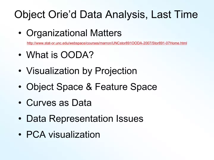
Object Orie’d Data Analysis, Last Time • Organizational Matters http://www.stat-or.unc.edu/webspace/courses/marron/UNCstor891OODA-2007/Stor891-07Home.html • What is OODA? • Visualization by Projection • Object Space & Feature Space • Curves as Data • Data Representation Issues • PCA visualization
Data Object Conceptualization Object Space Feature Space Curves Images Manifolds Shapes Tree Space Trees
Easy way to do these analyses • Matlab software (user friendly?) available: • http://www.stat.unc.edu/postscript/papers/marron/Matlab7Software/ • Download & put in Matlab Path: • General • Smoothing • Look first at: • curvdatSM.m • scatplotSM.m
Easy way to do these analyses Matlab software (user friendly?) available: http://www.stat.unc.edu/postscript/papers/marron/Matlab7Software/ ???????????????????????????? ??? Next time: Spend some time going through these As many students seem to want to use them
Time Series of Curves • Again a “Set of Curves” • But now Time Order is Important! • An approach: Use color to code for time Start End
Time Series Toy E.g. Explore Question: “Is Horizontal Motion Linear Variation?” Example: Set of time shifted Gaussian densities View: Code time with colors as above
T. S. Toy E.g., PCA View PCA gives “Modes of Variation” But there are Many… Intuitively Useful??? Like “harmonics”? Isn’t there only 1 mode of variation? Answer comes in 2-d scatterplots
T. S. Toy E.g., PCA Scatterplot • Where is the Point Cloud? • Lies along a 1-d curve in • So actually have 1-d mode of variation • But a non-linear mode of variation • Poorly captured by PCA (linear method) • Will study more later
Chemo-metric Time Series • Mass Spectrometry Measurements • On an Aging Substance, called “Estane” • Made over Logarithmic Time Grid, n = 60 • Each is a Spectrum • What about Time Evolution? • Approach: PCA & Time Coloring
Chemo-metric Time Series • Joint Work w/ E. Kober & J. Wendelberger • Los Alamos National Lab • Four Experimental Conditions: • Control • Aged 59 days in Dry Air • Aged 27 days in Humid Air • Aged 59 days in Humid Air
Chemo-metric Time Series, HA 27 • Raw Data: • All 60 spectra essentially the same • “Scale” of mean is much bigger than variation about mean • Hard to see structure of all 1600 freq’s • Centered Data: • Now can see different spectra • Since mean subtracted off • Note much smaller vertical axis
Chemo-metric Time Series, HA 27 • Data zoomed to “important” freq’s: • Raw Data: • Now see slight differences • Smoother “natural looking” spectra • Centered Data: • Differences in spectra more clear • Maybe now have “real structure” • Scale is important
Chemo-metric Time Series, HA 27 • Use of Time Order Coloring: • Raw Data: • Can see a little ordering, not much • Centered Data: • Clear time ordering • Shifting peaks? (compare to Raw) • PC1: • Almost everything? • PC1 Residuals: • Data nearly linear (same scale import’nt)
Chemo-metric Time Series, Control • PCA View • Clear systematic structure • Time ordering very important • Reminiscent of Toy Example • A clear 1-d curve in Feature Space • Physical Explanation?
Toy Data Explanations • Simple Chemical Reaction Model: • Subst. 1 transforms into Subst. 2 • Note: linear path in Feature Space
Toy Data Explanations • Richer Chemical Reaction Model: • Subst. 1 Subst. 2 Subst. 3 • Curved path in Feat. Sp. • 2 Reactions Curve lies in 2-dim’al subsp.
Toy Data Explanations • Another Chemical Reaction Model: • Subst. 1 Subst. 2 & Subst. 5 Subst. 6 • Curved path in Feat. Sp. • 2 Reactions Curve lies in 2-dim’al subsp.
Toy Data Explanations • More Complex Chemical Reaction Model: • 1 2 3 4 • Curved path in Feat. Sp. (lives in 3-d) • 3 Reactions Curve lies in 3-dim’al subsp.
Toy Data Explanations • Even More Complex Chemical Reaction Model: • 1 2 3 4 5 • Curved path in Feat. Sp. (lives in 4-d) • 4 Reactions Curve lies in 4-dim’al subsp.
Chemo-metric Time Series, Control • Suggestions from Toy Examples: • Clearly 3 reactions under way • Maybe a 4th??? • Hard to distinguish from noise? • Interesting statistical open problem!
Chemo-metric Time Series • What about the other experiments? Recall: • Control • Aged 59 days in Dry Air • Aged 27 days in Humid Air • Aged 59 days in Humid Air • Above results were “cherry picked”, • to best makes points • What about cases???
Scatterplot Matrix, Control Above E.g., maybe ~4d curve ~4 reactions
Scatterplot Matrix, Da59 PC2 is “bleeding of CO2”, discussed below
Scatterplot Matrix, Ha27 Only “3-d + noise”? Only 3 reactions
Scatterplot Matrix, Ha59 Harder to judge???
Object Space View, Control Terrible discretization effect, despite ~4d …
Object Space View, Da59 OK, except strange at beginning (CO2 …)
Object Space View, Ha27 Strong structure in PC1 Resid (d < 2)
Object Space View, Ha59 Lots at beginning, OK since “oldest”
Problem with Da59 What about strange behavior for DA59? Recall: PC2 showed “really different behavior at start” Chemists comments: Ignore this, should have started measuring later…
Problem with Da59 But still fun to look at broader spectra
Chemo-metric T. S. Joint View • Throw them all together as big population • Take Point Cloud View
Chemo-metric T. S. Joint View • Throw them all together as big population • Take Point Cloud View • Note 4d space of interest, driven by: • 4 clusters (3d) • PC1 of chemical reaction (1-d) • But these don’t appear as the 4 PCs • Chem. PC1 “spread over PC2,3,4” • Essentially a “rotation of interesting dir’ns” • How to “unrotate”???
Chemo-metric T. S. Joint View Interesting Variation: Remove cluster means Allows clear comparison of within curve variation
Chemo-metric T. S. Joint View • Interesting Variation: • Remove cluster means • Allows clear comparison of within curve variation: • PC1 versus others are quite revealing • (note different “rotations”) • Others don’t show so much
Demography Data Joint Work with: Andres Alonso Univ. Carlos III, Madrid • Mortality, as a function of age • “Chance of dying”, for Males, in Spain • of each 1-year age group • Curves are years • 1908 - 2002 • PCA of the family of curves
Demography Data • PCA of the family of curves for Males • Babies & elderly “most mortal” (Raw) • All getting better over time (Raw & PC1) • Except 1918 - Influenza Pandemic • (seeColor Scale) • Middle age most mortal (PC2): • 1918 • Early 1930s - Spanish Civil War • 1980 – 1994 (then better) auto wrecks • Decade Rounding (several places)
Demography Data • PCA for Females in Spain • Most aspects similar • (seeColor Scale) • No War Changes • Steady improvement until 70s (PC2) • When auto accidents kicked in
Demography Data • PCA for Males in Switzerland • Most aspects similar • No decade rounding (better records) • 1918 Flu – Different Color (PC2) • (seeColor Scale) • No War Changes • Steady improvement until 70s (PC2) • When auto accidents kicked in
Demography Data • Dual PCA • Idea: Rows and Columns trade places • Terminology: from optimization • Insights come from studying “primal” & “dual” problems