Download
1 / 55
1k likes | 2.41k Views
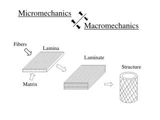
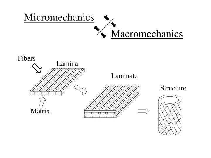
Micromechanics. Macromechanics. Fibers. Lamina. Laminate. Structure. Matrix. Micromechanics.

E N D
Micromechanics Macromechanics Fibers Lamina Laminate Structure Matrix
Micromechanics The analysis of relationships between effective composite properties (i.e., stiffness, strength) and the material properties, relative volume contents, and geometric arrangement of the constituent materials.
Micromechanics - Stiffness • Mechanics of materials models – Simplifying assumptions make it unnecessary to specify details of stress and strain distribution – fiber packing geometry is arbitrary. Use average stresses and strains.
Micromechanics - Stiffness • Theory of elasticity models - “Actual” stress and strain distributions are used – fiber packing geometry taken into account. • Closed form solutions • Numerical solutions such as finite element • Variational methods (bounds)
Volume Fractions fiber volume fraction matrix volume fraction void volume fraction Where (3.2) composite volume
Weight Fractions fiber weight fraction matrix weight fraction Where composite weight Note: weight of voids neglected
Densities density (3.6) “Rule of Mixtures” for density
Alternatively, (3.8) Eq. (3.2) can be rearranged as (3.9)
Above formula is useful for void fraction estimation from measured weights and densities. Typical void fractions: Autoclaved cured composite: 0.1% - 1% Press cured w/o vacuum: 2 - 5%
Measurements typically involve weight fractions, which are related to volume fractions by (3.10) and (3.12)
Fiber s s d s d s Representative area elements for idealized square and triangular fiber packing geometries. Square array Triangular array
Fiber volume fraction – packing geometry relationships Square array: (3.14) (3.15) When s=d,
Fiber volume fraction – packing geometry relationships Triangular Array: (3.16) (3.17) When s=d,
Fiber volume fraction – packing geometry relationships • Real composites: Random fiber packing array Unidirectional: Chopped: Filament wound: close to theoretical
Photomicrograph of carbon/epoxy composite showing actual fiber packing geometry at 400X magnification
Voronoi cell and its approximation. (From Yang, H. and Colton, J.S. 1994. Polymer Composites, 51, 34–41. With permission.) Random nature of fiber packing geometry in real composites can be quantified by the use of the Voronoi cell. Each point within the space of a Voronoi cell for a particular fiber is closer to the center of that fiber than it is to the center of any other fiber s Voronoi cells Equivalent square cells, with Voronoi cell size, s
Typical histogram of Voronoi distances and corresponding Wiebull distribution for a thermoplastic matrix composite. (From Yang, H. and Colton, J.S. 1994. Polymer Composites, 51, 34–41. With permission.)
Elementary Mechanics of Materials Models for Effective Moduli • Fiber packing array not specified – RVE consists of fiber and matrix blocks. • Improved mechanics of materials models and elasticity models do take into account fiber packing arrays.
Assumptions: • Area fractions = volume fractions • Perfect bonding at fiber/matrix interface – no slip • Matrix is isotropic, fiber can be orthotropic • Fiber and matrix linear elastic • Lamina is macroscopically homogeneous, linear elastic and orthotropic
Concept of an Effective Modulus of an Equivalent Homogeneous Material. Heterogeneous composite under varying stresses and strains Stress, Strain, Equivalent homogeneous material under average stresses and strains Stress Strain
Representative volume element and simple stress states used in elementary mechanics of materials models
Representative volume element and simple stress states used in elementary mechanics of materials models Longitudinal normal stress Transverse normal stress In-plane shear stress
Average stress over RVE: (3.19) Average strain over RVE: (3.20) Average displacement over RVE: (3.21)
Longitudinal Modulus RVE under average stress governed by longitudinal modulus E1. Equilibrium: Note: fibers are often orthotropic. Rearranging, we get “Rule of Mixtures” for longitudinal stress (3.22) Static Equilibrium (3.23)
Hooke’s law for composite, fiber and matrix Stress – strain Relations (3.24) So that: (3.25)
Assumption about average strains: Geometric Compatibility (3.26) Which means that, (3.27) “Rule of Mixtures” – generally quite accurate – useful for design calculations
Variation of composite moduli with fiber volume fraction Eq. 3.27 Eq. 3.40 Predicted E1 and E2 from elementary mechanics of materials models
Variation of composite moduli with fiber volume fraction Comparison of predicted and measured E1 for E-glass/polyester. (From Adams, R.D., 1987. Engineered Materials Handbook, Vol. 1, Composites, 206–217.)
Strain Energy Approach (3.28) Where strain energy in composite, fiber and matrix are given by, (3.29a) (3.29b) (3.29c)
Strain energy due to Poisson strain mismatch at fiber/matrix interface is neglected. Let the stresses in fiber and matrix be defined in terms of the composite stress as: (3.30) Subst. in “Rule of Mixtures” for longitudinal stress: (3.23)
Or (3.31) Combining (3.30), (3.24) & (3.29) in (3.28), (3.32) Solving (3.31) and (3.32) simultaneously for E-glass/epoxy with known properties: Find a1 and b1, then
Transverse Modulus RVE under average stress Response governed by transverse modulus E2 Geometric compatibility: From definition of normal strain, (3.34) (3.35)
Thus, Eq.(3.34) becomes (3.36) Or (3.37) Where 1-D Hooke’s laws for transverse loading: (3.38)
Where Poisson strains have been neglected. Combining (3.37) and (3.38), (3.39) Assuming that We get (3.40)
- “Inverse Rule of Mixtures” – Not very accurate - Strain energy approach for transverse loading, Assume, (3.41) Substituting in the compatibility equation (Rule of mixture for transverse strain), we get (3.42)
Then substituting these expressions for and in (3.28) We get (3.43) Solving (3.42) and (3.43) simultaneously for a2 and b2, we get for E-glass/epoxy,
In-Plane Shear Modulus, G12 • Using compatibility of shear displacement and assuming equal stresses in fiber and matrix: (Not very accurate) (3.47) Major Poisson’s Ratio, υ12 • Using compatibility in 1 and 2 directions: • (Good enough for design use) (3.45)
Design Equations • Elementary mechanics of materials Equations derived for G12 and E2 are not very useful – need to develop improved models for G12 and E2.
Improved Mechanics of Materials Models for E2 and G12 Mechanics of materials models refined by assuming a specific fiber packing array. Example: Hopkins – Chamis method of sub-regions RVE
Convert RVE with circular fiber to equivalent RVE having square fiber whose area is the same as the circular fiber. RVE Sub Region A A sf A Sub Region B s sf B B d A Sub Region A A Division of representative volume element into sub regions based on square fiber having equivalent fiber volume fraction.
s sf sf Equivalent Square Fiber: (from ) (3.48) Size of RVE: (3.49) For Sub Region B:
Following the procedure for the elementary mechanics of materials analysis of transverse modulus: (3.50) but (3.51) So that (3.52)
For sub regions A and B in parallel, (3.53) Or finally (3.54) Similarly,
Simplified Micromechanics Equations (Chamis) Only used part of the analysis for sub region B in Eq. (3.52): (3.52) Fiber properties Ef2 and Gf12 in tables inferred from these equations.
Semi empirical Models Use empirical equations which have a theoretical basis in mechanics Halpin-Tsai Equations (3.63) Where (3.64)
And curve-fitting parameter 2 for E2 of square array of circular fibers 1 for G12 As Rule of Mixtures As Inverse Rule of Mixtures