Download
1 / 48
520 likes | 815 Views
Conditional probability and Statistically Independent Events. Introduction. In many real-world “experiments”, the outcomes are not completely random since we have some prior knowledge.

E N D
Introduction • In many real-world “experiments”, the outcomes are not completely random since we have some prior knowledge. • Knowing that it has rained the previous two days might influence our assignment of the probability of sunshine for the following day. • The probability that an individual chosen from some general population weights more than 90 kg, knowing that his height exceeds 6ft. • We might inquire the probability of obtaining a 4, if it is known that the outcome is an even number
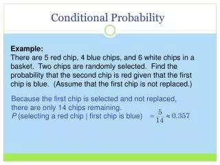
Joint Events and Conditional Probability • The event of interest A = {4}, and the event describing our prior knowledge is an even outcome or B = {2,4,6} • Note, conditional probability does not address the reasons for the prior information. The odd outcomes are shown as dashed lines and are to be ignored, then P[A] = 9/25 9 is the total number of 4’s 25 is the number of 2’s, 4’s and 6’s
Joint Events and Conditional Probability Determine the probability of A = {1,4}, knowing that outcome is even. • We should use to make sure we only count the outcomes that can occur in light of our knowledge of B. • Let S = {1,2,3,4,5,6} be the sample space, and NS its size, the probability of A given B is The conditional probability is denoted by and defined as
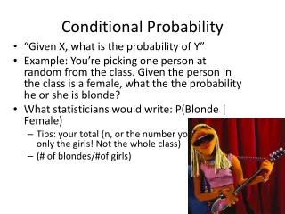
Height and weights of college students • A population of college students have heights H and weights W which are grouped into ranges. • Determine the probability of the event A that the student has a weight in the range 130-160 lbs. • Determine the probability of the event A, given that the student has height less than 6’ (event B). Probability changed
Marginal probability • The probabilities P[Hi] are called the marginal probabilities since they are written in the margin of the table. • If we were to sum along the columns, then we would obtain the marginal probabilities for the weights or P[Wj].
Conditional probability • The probability of the event A that the student has a weight in the range 130-160 lbs. • Probability of even A, given that the students height is less than 6’, the probability of the event has changed to • Probability of even A, given that the students height is greater than 6’, the probability of the event has changed to
Conditional probability • In general Statistically independent
A compound experiment • Two urns contain different proportions of red and black balls. • Urn 1 has a proportions p1 of red balls and 1-p1of black balls. • Urn 2 has proportions of p2and 1-p2red balls and black balls. • An urn is chosen at random, followed by the selection of a ball. • Find a probability that red ball is selected. • Do B1 = {urn 1 chosen} and B2 = {urn 2 chosen} partition the sample space? • We need to show and .
Probability of error in a digital communication system • In digital com. System a “0” or “1” is transmitted to a receiver. • Either bit is equally likely to occur so that prior probability of ½ is assumed. • At the receiver a decoding error e can be made due to channel noise, so that a 0 may be mistaken for a 1 and vice versa. Similar to urn problem
Monty Hall problem Behind one door there is a new car, while the others concealed goats. http://www.youtube.com/watch?v=mhlc7peGlGg The contestant would first have the opportunity to choose a door, but it would not be opened. Monty would then choose the door with a goat. The contestant was given is given the option to either open the door that was chosen or open the other door. Question is open of switch?
Monty Hall problem • Assume the car is behind door 1. • Define the events Ci = {contestant initially chooses door i} for i = 1,2,3 and Mj= {Mounty opens door j} for j = 1,2,3. • Determine the joint probabilities P[Ci, Mj] by using P[Ci, Mj] = P[Mj|Ci]P[Ci] • Since the winning door is never chosen by Monty, we have P[M1|Ci] = 0. Also Monty never opens the door initially chosen by the contestant so that P[Mi|Ci] = 0.Then • P[M2 | C3] = P[M3 | C2] = 1 (contestant chooses losing door) • P[M3 | C1] = P[M2| C1] = ½ (contestant chooses winning door) • P[Ci] = 1/3
Statistically Independent Events • Two events A and B are said to be statistically independent if P[A|B] = P[A] • Thus • Knowing that B has occurred does in fact affect that possible outcomes. However, it is the ratio of to that remains the same.
Statistical independence does not mean one event does not affect another event • If a fair die is tossed, the probability of a 2 or a 3 is P[A={2,3}] = 1/3. Now assume we know the outcome is an even number or B = {2,4,6}. Recomputing the probability • The event has half as many elements as A, but the reduced sample space S’ = B also has half as many elements.
Statistically Independent Events: Important points • We need only know the marginal probabilities or P[A], P[B] to determine the join probability . • Hence, we need only know the marginal probabilities or P[A], P[B]. • Statistical independence has a symmetry property. If A is independent of B, then B must be independent of A since commutative property A is independent of B
Statistical independent events are different than mutually exclusive events • If A and B are mutually exclusive and B occurs, then A cannot occur. P[A|B] = 0 • If A and B are statistically independent and B occurs, then P[A|B] = P[A]. The probabilities are only the same if P[A] = 0. • The conditions of mutually exclusivity and independence are different. Mutually exclusive events Statistically independent events
Statistically Independent three or more Events • Three events are defined to be independent if the knowledge that any one or two of the events has occurred does not affect the probability of the third event. • Note that if B and C has occurred, then by definition has occurred. • The full set of conditions is • These conditions are satisfied if and only if Pairwise independent
Statistically Independent three or more Events • We need because • In general, events E1, E2, …, ENare defined to be statistically independent if • Statistical independence allows us to compute joint probabilities based on only the marginal probabilities.
Probability chain rule • We can still determine joint probabilities for dependent events, but it becomes more difficult. Consider three events • It is not always an easy matter to find conditional probabilities. • Example: Tossing a fair die • If we toss a fair die, then the probability of the outcome being 4 is 1/6. • Let us rederive this result by using chain rule. Letting • A = {event number} = {2, 4, 6} • B = {numbers > 2} = {3, 4, 5, 6} • C = {numbers < 5} = {1, 2, 3, 4} • We have that ABC = {4}. Applying chain rule and noting that BC = {3,4} we have chain rule
Bayes’ Theorem • Recall conditional probability • Substituting from to we obtain obtain Bayes’ theorem. • By knowing the marginal probabilities and conditional probability we can determine the other conditional probability . • The theorem allows us to perform inference or to assess the validity of an event when some other event has been observed.
Bayes’ Theorem: Example • If an urn containing an unknown composition of balls is sampled with replacement and produces an outcome of 10 red balls, what are we to make of this? • Are all balls red? • Is the urn fair (half red and half black)? ? • To test that the urn is a “fair” one, we determine the probability of a fair urn given that 10 red balls have just drawn. • Usually we compute the probability of choosing 10 red balls given a fain urn, now are going “backwards”. Now we are given the outcomes and wish to determine the probability of a fair urn.
Bayes’ Theorem: Example • We believe that the urn is fair with probability 0.9 (from our past experience). B = {fair urn}, so P[B] = 0.9. • If A = {10 red balls drawn}, we wish to determine P[B|A]. • This probability is our reassessment of the fair urn in light of the new evidence (10 red balls drawn). • According to Byes theorem we need conditional probability P[A|B]. P[A|B] is the probability of drawing 10 successive red balls from an urn with p = ½. • By now we know P[B], P[A|B]. We need to find P[A].
Bayes’ Theorem: Example • P[A]can be found using the law of total probability as • And thus only need to be determined. This is the conditional probability of drawing 10 red balls from a unfair urn (assume all balls in the urn are red) and thus . • The posterior probability (after 10 red balls have been drawn) • The odds ratio is interpreted as the odds against the hypothesis of a fair urn. Reject fair urn hypothesis
Multiple Experiments • The experiment of the repeated tossing coin can be view as a succession of subexperiments(single coin toss). • Assume a coin is tossed twice and we wish to determine P[A], where A ={(H,T)}. For a fair coin it is ¼ since we assume that all 4 possible outcomes are equally probable. • If the coin had P[{H}]=0.99, the answer is not straight forward. How to determine such probabilities?
Multiple Experiments • Consider the experiment composed of two separate subexperiments with each subexperiment having a sample space S1 = {H, T}. The sample space of the overall experiment is • P[complicated events] by determining P[events defined on S1]. • The statement is correct if we Assume that the subexperiments are independent. • So what is P[A]= P[(H,T)] is a coin with P[{H}] = p. • This event is define on the sample space of 2-tuples, which is S.
Multiple Experiments • Subexperiments are independent, hence P[(H,T)] = P[H1][T2], • We can determine P[H1] either as P[(H,H), (H,T)] or as P[H] due to independence assumption. • P[H] is a marginal probability and is equal to P[(H,H)] + P[(H,T)] . • P[H1] = p • P[T2] = 1 – p. • and finally P[(H,T)] = p(1-p). • Generally, if we have M independent subexperiments, with Ai an event described for experiment i, then the joint event has probability Equivalence to statistical independence of events defined on the same sample space.
Bernoulli Sequence • Any sequence of M independent subexperiments with each subexperiment producing two possible outcomes is called a Bernoulli sequence • Typically, for a Bernoulli trial P[0] = 1 – p, P[1] = p.
Binomial Probability Law • Assume that M independent Bernoulli are carried out. • We wish to determine the probability of k’s (successes) and M-k0’s. • Thus, each successful outcome has a probability of pk(1 - p)M-k. • The total number of successful outcomes is the number of ways k 1’s may be place in the M-tuple i.e. . • Hence, we have Binomial law M = 10, p = 0.5 M = 10, p = 0.7
Geometric Probability Law • If we let k be the Bernoulli trial for which the first success is observed, then the event of interest us the simple even (f,f,…,f,s), where s, f denote success and failure. • The probability of the first success at trial k is therefore • The first success is always most likely to occur on the first trial(k = 1) • The average number of trials required for success is 1/p. p = 0.5 p = 0.25
Example: Telephone calling • A fax machine dials a phone number that is typically busy 80% of the time. What is the probability that the fax machine will have to dial the number 9 times? • The number of times the line is busy can be considered the number of failures with each failure having a probability of 1- p = 0.8. • If the number is dialed 9 times, then the first success occurs for k = 9 and P[9] = (0.8)8(0.2) = 0.0336
NoindependentSubexperiments • The assumption of independence can sometimes be unreasonable. In the absence of independence, the probability would found by using chain rule. P[A] = P[AM|AM-1,…,A1]P[AM-1|AM-2,…,A1]…P[A2|A1]P[A1] • Dependent Bernoulli trials • Assume we have two coins. One fair and the other is weighted (p≠1/2) • We randomly choose a coin and toss it. • If it comes up head, we choose the fair coin to use on the next trial. • If it comes up tails, we choose the weighted coin to use on the next trial. M = 100, p = 0.25 M = 100, p = 0.5
Markov Sequence • The dependency between trials is due only to the outcome of the (i - 1) trial affecting the outcome of the ith trial. • The previous outcome is called the state of the sequence. State probability diagram • The Bernoulli sequence, in which the probability of trials i depend only on the outcome of the previous trial, is called a Markov sequence. P[Ai|Ai-1, Ai-2,…,A1] = P[Ai|Ai-1] P[A] = P[AM|AM-1]P[AM-1|AM-2]…P[A2|A1]P[A1] state transition
Markov Sequence: example • We wish to determine the probability of N = 10 tails in succession or the event A = {(0,0,0,0,0,0,0,0,0,0)}. • If the coin is fair, then P[A] = (1/2)10= 0.000976, • If the coin is weighted (P[1] = ¼ ), then • but P[Ai|Ai-1] = P[0|0] = P[tail | weightedcoin] = ¾ for i = 2,3,…,10. • Initial choice of the coin is random, hence 48 times larger
Trellis diagram • The probability of any sequence is found by tracing the sequence values through the trellis diagram and multiplying the probabilities for each branch together. • The sequence 1,0,0 has a probability of (3/8)(1/2)(3/4).
Real-world example: Cluster recognition • We wish to determine if a cluster of event has occurred. • By cluster we mean that more occurrences of an event are observed than would normally be expected. Hit rate is 29/2500 = 1.16%
Real-world example: Cluster recognition • The shaded area exhibit more hits than the expected 145 x 0.0116 = 1.68 number. Is this cluster? • Let’s apply Bayesian approach and calculate odds ration to answer the question. • B = {cluster} and • A = {observed data} • P[A] cancelles out
Real-world example: Cluster recognition • We need to determine • P[B] is prior probability, since we believe a cluster is quite unlikely, we assign probability of 10-6. • The probability of the observed data if there is no cluster is calculated using Bernoulli sequence (array). If M cells contained in the supposed cluster area (M = 145) then the probability of k hits is • Setting pnc = 0.01, which is less then 0.0116 the hit rate, and denotes the probability of no cluster. • The probability that there is a cluster is set to pc = 0.1. 11/145 = 0.07
Real-world example: Cluster recognition • Which results in an odds ratio of • Mainly the influence of the small prior probability of a cluster, P[B]=10-6, that has resulted in the greater than unity odds ratio. Reject cluster hyp.
Practice problems 1. 2.
Practice problem 3. 4.
Practice 5. 6. 7.
Practice 8.
Practice 9. In a culture used for biological research the growth of unavoidable bacteria occasionally spoils results of an experiment that requires at least three out of five cultures to be unspoiled to obtain a single datum point. Experience has shown that about 5 of every 100 cultures are randomly spoiled by the bacteria. If the experiment requires three simultaneously derived , unspoiled data points for success, find the probability of success for any given set of 15 cultures (three data pointes of five cultures each).
Homework problems 1. 2. 3.
Homework 4. 5. 6. 7*.