Download
1 / 55
550 likes | 757 Views
Managerial Economics. Session 2. Cost Analysis and Supply. Professor Changqi Wu. Topics for Today. Production and Cost Cost Concepts Cost Analysis Firm’s Production Decision Supply Curve Market Mechanism. 1. Production and Cost.

E N D
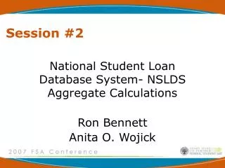
Managerial Economics Session 2 Cost Analysis and Supply Professor Changqi Wu
Topics for Today • Production and Cost • Cost Concepts • Cost Analysis • Firm’s Production Decision • Supply Curve • Market Mechanism Cost analysis
1. Production and Cost • Production process utilizes productive inputs to produce useful output for buyers • Categories of production inputs • labor (skilled and unskilled) • capital • technology • Management skills Cost analysis
Production Function • Production Function indicates the highest output that a firm can produce for every specified combination of inputs given the state of technology. • The production function for two inputs: Q = F(K,L) Q = Output, K = Capital, L = Labor Cost analysis
AP = slope of line from origin to a point on TP, lines B, & C. • MP = slope of a tangent to any point on the TP line, lines A, C, D. Production with One Variable Input Output per Month Output per Month D 112 Marginal product 30 C Average product Total product E 20 60 B 10 A Labor per Month Labor per Month 0 1 2 3 4 5 6 7 8 9 10 1 10 9 0 2 3 4 5 6 7 8
Diminishing Marginal Returns • As the use of an input increases in equal increments, a point will be reached at which the resulting additions to output decreases (i.e. Marginal Product declines). Cost analysis
From Production to Cost • A production function measures the relationship between inputs and output. • To determine the optimal level of output, we must translate the production technology to dollar value of costs. Cost analysis
Cost is not Waste • A cost curve depicts the relationship between output and the most efficient way of producing that output. • A cost curve is the mirror image of the production function • Input price change moves cost curve • Technology change moves cost curve Cost analysis
Economic and Accounting Concepts of Cost • Accounting Cost • Actual expenses plus depreciation charges for capital equipment • Historical records • Economic Cost • Cost of utilizing economic resources in production, including opportunity cost • Forward looking Cost analysis
Opportunity Cost • Business decision making requires information on future alternative courses of action • Opportunity cost measures the forgone net revenue from the best alternative course of action • Example of opportunity cost: • Shanghai Petrochemicals Cost analysis
Shanghai Petrochemicals • Shanghai Petrochemicals is a listed company at the Stock Exchanges of both New York and Hong Kong. • Its 1994 Annual Report shows that the company made a profit of RMB 1.77 billion. • In that year Shanghai Petrochemicals bought 4.5 million ton of crude oil at the subsidized price of RMB670/ton while the crude oil price in the international market was at average RMB1100/ton. • Indirect cost savings due to the government subsidies amounted to RMB 1.93 billion. • The company actually lost RMB 150 million in that year. Cost analysis
2. Concepts of Cost • The total cost of production equals the fixed cost (the cost of the fixed inputs) plus the variable cost (the cost of the variable inputs) Cost analysis
Total cost is the vertical sum of FC and VC. TC Cost ($ per year) 400 VC Variable cost increases with production and the rate varies with increasing & decreasing returns. 300 200 Fixed cost does not vary with output 100 FC 50 Output 0 1 2 3 4 5 6 7 8 9 10 11 12 13 Total Cost Curves of a Firm Cost analysis
Average Total Cost • Average Total Cost (ATC) is the cost per unit of output, or average fixed cost (AFC) plus average variable cost (AVC). This can be written: Cost analysis
Marginal Cost • Marginal Cost (MC) is the cost of expanding output by one unit. Since fixed cost have no impact on marginal cost, it can be written as: Cost analysis
Unit Cost Curves Cost ($ per unit) 100 MC 75 50 ATC AVC 25 AFC Output (units/yr.) 1 0 2 3 4 5 6 7 8 9 10 11 Cost analysis
Fixed Cost and Sunk Cost • Expenditure that has been made and cannot be recovered. • Sunk cost should not influence a firm’s decision. • An example • A firm pays $500,000 of deposit for an option to buy a building. • The cost of the building is $5 million or a total of $5.5 million. • The firm finds another building for $5.25 million. • Which building should the firm buy? Cost analysis
3. Cost Analysis • Economy of scale • Economy of scope • Economy of experience • Economy of time Cost analysis
3.1 Economy of Scale • Economy of scale means… Average cost declines when the scale of production expands • Economy of scale may arise at different levels of production • product level, plant level, firm level • Economy of scale may arise at different aspects of business operations • production, marketing, R&D Cost analysis
Economy of Scale Unit Costs ($/unit) $10 $5 LAC (including cost of capital) Annual Sales Volume (units per year) 1000 4000 5000 Your current sales volume. Small firm’s current sales volume. MES Cost analysis
Sources of Economy of Scale • Production requires significant fixed inputs • indivisibility • Physical laws: the two third rule construction cost = k (throughput)2/3 • Economy of mass reserves • Specialized labor • Economy of scales in purchasing Cost analysis
Minimum Efficient Scale is ... the smallest production scale at which minimum unit cost is attained • Methods to assess MES in an industry • Statistical estimation of cost function • The survivor principle • Profitability and firm size • Engineering approach • MES may change when technology advances Cost analysis
Economy of Scale in Action • Take advantages of economy of scale • Building inventory • Contracting out • Developing backlog • Strategic implications of economy of scale Cost analysis
3.2 Economy of Experiences Unit Cost • Experience curves are characterized by their slope • (also called BCG slope or progress ratio) • Slope = by how much do unit costs fall • --- as a percentage of a baseline level --- when • cumulative output doubles. $1.00/unit $0.80/unit Experience Curve with 80% Slope Cumulative Production Volume (total number of units produced to date) 100 200 Cost analysis
Sources of Experience Effect • Labor efficiency • New processes and improved methods • Product redesign • Product standardization Cost analysis
Economy of Experience in Action • We can use experience curve to forecast cost changes • Forward pricing: pricing based on future cost • strategic effect: moving down quickly along experience curve to gain competitive advantage • Using pre-launch announcement to prevent rivals from taking advantage of economy of learning • A firms enjoying a experience based low cost should take measures to reduce employee turnovers Cost analysis
Economy of Experience in Action • Earlier-mover advantage refers to the idea that "the rich get richer” • Because your business unit has entered a market early (either by happenstance or superior foresight), your past success in the market sustains a dynamics whereby your cost or benefit advantage becomes more pronounced over time. Cost analysis
Economies of Scale Versus Learning • Production capacity • Time span Cost analysis
Economies of Scale A B AC1999 Learning C AC2000 Economies ofScale Versus Learning Cost ($ per unit of output) Output Cost analysis
3.3 Economy of Scope • Economy of scope exists when the total cost of a single firm with multiple products is lower than the sum of the total costs of two independent firms with each producing the a single product. • Examples: • Chicken farm--poultry and eggs • Automobile company--cars and trucks • Universal banking Cost analysis
Degree of Economies of Scope • The degree of economies of scope measures the savings in cost and can be written: • If SC > 0 -- Economies of scope • If SC < 0 -- Diseconomies of scope Cost analysis
3.4 Economy of Time • The Case of PC Market • Moore’s Law dominates • Highly competitive with modulization • Product life cycle is only 3 months • Price of components falls 50 % a year. One percent a week. Cost analysis
What is Dell doing? Price B1 B V1 Sales Line (price now fixed) V Time Line W A U X Rate of Price Decline X1 Y Rate of Price Decline Y1 Time Cost analysis
Implications • Can we apply the Dell model to other businesses? • Toyota introduced the build-to-order system in 1999 • Costs were lowed • Client satisfaction rose. Cost analysis
4. Output Decision and Supply Cost analysis
Choosing Output in the Short Run • A competitive firm acts as a price-taker, its marginal revenue is a horizontal line • P = D = MR = AR • Observations: • P = MR • MR = MC • P = MC Cost analysis
MC Lost profit for qq < q* Lost profit for q2 > q* A D AR=MR=P ATC C B AVC At q*: MR = MC and P > ATC q1 : MR > MC and q2: MC > MR and q0: MC = MR but MC falling q0 q1 q* q2 A Competitive FirmMaking a Positive Profit Price ($ per unit) 60 50 40 30 20 10 0 1 2 3 4 5 6 7 8 9 10 11 Output Cost analysis
MC ATC B C D P = MR A At q*: MR = MC and P < ATC Losses = P- AC) x q* or ABCD AVC F E q* A Competitive FirmIncurring Losses Price ($ per unit) Would this producer continue to produce with a loss? Output Cost analysis
Summary of Production Decisions • Profit is maximized when MC = MR • If P > ATC the firm is making profits. • If AVC < P < ATC the firm should produce at a loss. • If P < AVC < ATC the firm should shut-down. Cost analysis
Supply Curve • Supply curve depicts the relationship between price and quantity supplied • Supply curve depend on the time needed for production adjustment • Short-run supply curve replicates part of a firm’s marginal cost curve • Industry supply curve is horizontal add-up of individual firms’ supply curves Cost analysis
A Firm’s Supply Curve S = MC above AVC Price ($ per unit) MC ATC P2 AVC P1 P = AVC Shut-down Output q1 q2 Cost analysis
Observations • Supply is upward sloping due to diminishing returns. • Higher price compensates the firm for higher cost of additional output and increases total profit because it applies to all units. Cost analysis
S The short-run industry supply curve is the horizontal summation of the supply curves of the firms. MC1 MC2 MC3 P3 P2 P1 Industry Supply $ per unit Question: If increasing output raises input costs, what impact would it have on market supply? Quantity 0 2 4 5 7 8 10 15 21 Cost analysis
Supply Elasticity • Supply elasticity is Responsiveness of supply of a good to changes in price measured as % change of the supply for an item if the price changes by 1% • Property Price elasticity of supply > 0 Cost analysis
Producer Surplus • Firms earn a surplus on all but the last unit of output. • The producer surplus is the sum over all units produced of the difference between the market price of the good and the marginal cost of production. • Producer surplus is very sensitive to price changes Cost analysis
At q* MC = MR. Between 0 and q , MR > MC for all units. Producer Surplus MC AVC B A P Alternatively, VC is the sum of MC or ODCq* . R is P x q*or OABq*. Producer surplus = R - VC or ABCD. D C q* Producer Surplus of a Firm Price ($ per unit of output) 0 Output Cost analysis
5. The Market Mechanism Characteristics of a competitive market • Many buyers and sellers in the marketplace. • All sellers sell identical products. • Free entry and exit. • Perfect information Cost analysis
The Market Mechanism • A market is at equilibrium when market demand equals market supply • When demand or supply conditions change, market equilibrium will change. • Price may deviate from market equilibrium. When that happens, market participants react to the new market conditions. That restores the market equilibrium. Cost analysis
S The curves intersect at equilibrium, or market- clearing, price. At P0the quantity supplied is equal to the quantity demanded at Q0 . P0 D Q0 The Market Equilibrium Price ($ per unit) Quantity Cost analysis
Price ($ per unit) S Surplus P1 Assume the price is P1 , then: 1) Qs : Q1 > Qd : Q2 2) Excess supply is Q1:Q2. 3) Producers lower price. 4) Quantity supplied decreases and quantity demanded increases. 5) Equilibrium at P2Q3 P2 D Quantity Q2 Q3 Q1 The Market Mechanism Cost analysis