Download

1 / 29
330 likes | 816 Views
Detailed Production Planning & Shop-Floor Control. Dealing with the Problem Complexity through Decomposition. Corporate Strategy. Aggregate Unit Demand. Aggregate Planning. (Plan. Hor.: 1 year, Time Unit: 1 month). Capacity and Aggregate Production Plans. End Item (SKU) Demand.

E N D
Dealing with the Problem Complexity through Decomposition Corporate Strategy Aggregate Unit Demand Aggregate Planning (Plan. Hor.: 1 year, Time Unit: 1 month) Capacity and Aggregate Production Plans End Item (SKU) Demand Master Production Scheduling (Plan. Hor.: a few months, Time Unit: 1 week) SKU-level Production Plans Manufacturing and Procurement lead times Materials Requirement Planning (Plan. Hor.: a few months, Time Unit: 1 week) Component Production lots and due dates Shop floor-level Production Control Part process plans (Plan. Hor.: a day or a shift, Time Unit: real-time)
The (Master) Production Scheduling Problem Capacity Consts. Company Policies Product Charact. Economic Considerations Placed Orders MPS Master Production Schedule: When & How Much to produce for each product Forecasted Demand • Current and Planned • Availability, eg., • Initial Inventory, • Initiated Production, • Subcontracted quantities Planning Horizon Time unit Capacity Planning
Grain cracking (1 milling machine) Mashing (1 mashing tun) Boiling (1 brew kettle) Fermentation (3 40-barrel ferm. tanks) Filtering (1 filter tank) Bottling (1 bottling station) MPS Example: Company Operations Fermentation Times:
Inventory Position: IPi = max{IPi-1,0}+ SRi+BNRi -Di (Material Balance Equation) (IPi-1)+ Di i SRi+BNRi IPi Computing Inventory Positions and Net Requirements Net Requirement: NRi = abs(min{0, IPi})
Computing Spoilage and Modified Inventory Position Spoilage: SPi = max{0, IPi-1-(SRi-1+SRi-2+…+SRi-sl+1) -(BNRi-1+BNRi-2+…+BNRi-sl+1)} Inventory Position: IPi = max{IPi-1,0}+ SRi+BNRi -Di-SPi (Material Balance Equation) (IPi-1)+ Di i SPi SRi+BNRi IPi
The Driving Logic behind the Empirical Approach • Initial Inventory Position • Scheduled Receipts due to initiated production or subcontracting Demand Availability: Compute Future Inventory Positions Net Requirements Future inventories Lot Sizing Scheduled Releases Resource (Fermentor) Occupancy Product i Revise Prod. Reqs Feasibility Testing Schedule Infeasibilities Master Production Schedule
MRP Planned Order Releases MPS Current Availabilities Priority Planning The “MRP Explosion” Calculus Lot Sizing Policies Lead Times BOM
Example: The (complete) MRP Explosion Calculus Item BOM: Alpha B(1) C(1) D(2) C(2) E(1) F(1) E(1) F(1) Item Levels: Level 0: Alpha Level 1: B Level 2: C, D Level 3: E, F
The “MRP Explosion” Calculus External Demand Level 0 Capacity Planning Initial Inventories Level 1 Level 2 Scheduled Receipts Level N Planned Order Releases Gross Requirements
Computing the item Scheduled Releases Safety Stock Requirements Lot Sizing Policy Lead Time Gross Reqs Planned Order Releases Parent Sched. Rel. Planned Order Receipts Net Reqs Synthesizing item demand series Projecting Inv. Positions and Net Reqs. Lot Sizing Time- Phasing Item External Demand Scheduled Receipts Initial Inventory
Lot Sizing • If affordable, a lot-for-lot (L4L) policy will incur the lowest inventory holding costs and it will maintain a smoother production flow. • Possible reasons for departure from a L4L policy: • High set up times and costs =>need for serial process batching to control the capacity losses • Processes that require a large production volume in order to maintain a high utilization (e.g., fermentors, furnaces, etc.) => need for parallel process batching • Selection of a pertinent process batch size • It must be large enough to maintain feasibility of the production requirements • It must control the incurred • inventory holding costs, and/or • part delays (this is a measure of disruption to the production flow caused by batching) • Move or transfer batches:The quantities in which parts are moved between the successive processing stations. • They should be as small as possible to maintain a smooth process flow
Some Lot Sizing Methods employed in the traditional MRP framework • Main focus: Balance set-up and holding costs • Wagner-Whitin Algorithm for dynamic Lot Sizing • Economic Order Quantity (EOQ): Compute a lot size using the EOQ formula with the demand rate D set equal to the average of the net requirements observed over the considered planning horizon. • Periodic Order Quantity (POQ): Compute T = round(EOQ/D), and every time you schedule a new lot, size it to cover the net requirements for the subsequent T periods. • Silver-Meal (SM): Every time you start a new lot, keep adding the net requirements of the subsequent periods, as long as the average (setup plus holding) cost per period decreases. • Least Unit Cost (LUC): Every time you start a new lot, keep adding the net requirements of the subsequent periods, as long as the average (setup plus holding) cost per unit decreases. • Part Period Balancing (PPB): Every time you start a new lot, add a number of subsequent periods such that the total holding cost matches the lot set up cost as much as possible.
Finite-Capacity Planning & Scheduling in the MRP II / ERP context: Load Reports (Example) Available resource time 150 100 50 8 1 2 3 Periods 4 5 6 7
Finite-Capacity Planning & Scheduling in the MRP II / ERP context: More Systematic Approaches • Bottleneck-based scheduling in a cellular manufacturing context (Goldratt’s Theory of Constraints approach): • Each part (family) has its own production cell with a well-defined bottleneck resource. • Production is scheduled on the bottleneck resource and the schedule for the other resources are organized around this schedule by taking consideration the expected lead times. • Typically, a “cushion” of extra workload is maintained at the bottleneck in order to prevent its starvation, in case of any disruptions in the upstream processes. • If the bottleneck supports the production of more than one part types, a “single-machine” scheduling problem arises naturally. This is addressed by selecting an appropriate dispatching rule. • Earliest Due Date (EDD) => minimizes maximum lateness (tardiness) • Least slack (LS), where slack = difference between job due date and expected completion time => tend to reduce average tardiness • Shortest Processing Time (SPT) => minimizes average flowtime at the bottleneck, and (by Little’s law) average WIP • Other heuristics addressing different problem variations including weighted performance measures, non-zero release times, etc.
Finite-Capacity Planning & Scheduling in the MRP II / ERP context: More Systematic Approaches (cont.) • Cases where the previous approach is not effective: • There are more than one capacity-constrained resource • Bottlenecks are shifting depending on the product mix • There are operations involving parallel process batching • Process routes are non-linear (e.g., due to routing flexibility, re-entrance, extensive need for rework) • Remark: The semiconductor manufacturing operational context is a typical example of all of the above. • A more global view of the system operations is necessary in order to support effective and efficient scheduling. • Possible approaches • Employ a set of pertinently selected dispatching rules at the different (critical) resources, and assess its efficacy through simulation (possibly maintain a bank of such rules for different operational conditions – meta-heuristics) • Generate efficient (not necessarily optimal) global schedules by employing an approach that searches for such a schedule in the space of feasible schedules
Typical approaches employed in the solution of the job shop scheduling problem • Branch & Bound (B&B): Constructs all possible schedules incrementally, fathoming options that are clearly suboptimal to some other options. Can generate optimal schedules but it is very time consuming. • Beam search: Similar to B&B, but it employs additional heuristics to increase fathoming. • Local search techniques: Given an initially constructed schedule, try to identify an improved schedule that is obtained from the original one through a localized change (e.g., through the change of the order of two jobs on a single machine); repeat. Also, need a mechanism to avoid local optima. • Simulated annealing: Seeks to avoid local optima by maintaining a non-zero probability for transitioning to an inferior schedule. However, this probability is reduced with the passage of time. • Tabu search: Seeks to avoid local optima by pronouncing certain schedule changes as taboo (these changes are apparent improvements that might attract the schedule back to a local optimum) • Genetic algorithms: Maintains an entire set of schedules at each iteration, and it updates this set by replacing schedules of inferior performance with new schedules resulting from the “combination” of the most efficient schedules currently available; the synthesis of such new schedules is known as “crossover”. Also, “mutation” provides additional schedules resulting from the local modification of some single schedules.
Typical approaches employed in the solution of the job shop scheduling problem • The “shifting bottleneck” heuristic: Originally developed for minimizing the schedule makespan, but there are also additional versions, e.g., for minimizing total weighted tardiness (c.f. Pinedo, Scheduling: Theory, Algorithms and Systems, Prentice Hall, 2002) • Start with a simple schedule that observes only the precedence constraints imposed by the job process routes and ignores completely the impact of the part contest for the various workstations. • Repeat • Identify the “bottleneck” machine that causes the highest disruption (delay) to the currently developed schedule, by solving a “single machine, maximum lateness with release times” problem, for each machine; the release times and the due dates for this max lateness problem are determined by the “critical path” in the currently available schedule. • Enter the schedule of the identified bottleneck to the current schedule. • Reschedule all the previously scheduled machines to improve the overall schedule efficiency; each of these rescheduling problems is another “single machine, maximum lateness with release times” problem, induced by the current schedule. • until all machines have been introduced to the running schedule.
Pegging and Bottom-up Replanning (borrowed from Heizer and Render)
Some Limitations of MRP-based Planning • The employment of fixed nominal lead times • This problem is mitigated in case of a stable operational environment where past experience and / or approximate formal models can provide insight for setting lead times • Lead time assessment is also facilitated by a well-structured, cellular shop-floor • Lack of an inherent mechanism for detecting and managing shop-floor congestion – a purely “Push” approach • However, it is possible to combine the planning visibility offered by the MRP explosion calculus with more sophisticated production control mechanisms that take advantage of the existing technology of Manufacturing Execution Systems (MES). • Possible system nervousness due to re-planning and the applied lot sizing policies • Potential remedies • Firm orders • Time fences • L4L planning whenever possible