Download
1 / 25
250 likes | 466 Views
Quantitative Methods in Social Research 2010/11. Week 2 (Morning) A novice’s guide to quantitative analysis . Examining quantitative data. Quantitative measures are typically referred to as variables.

E N D
Quantitative Methods in Social Research 2010/11 Week 2 (Morning) A novice’s guide to quantitative analysis
Examining quantitative data • Quantitative measures are typically referred to as variables. • Some variables are generated directly via the data generation process, but other, derived variables may be constructed from the original set of variables later on. • As the next slide indicates, variables are frequently referred to in more specific ways.
Cause(s) and effect…? • Often, one variable (and occasionally more than one variable) is viewed as being the dependent variable. • Variables which are viewed as impacting upon this variable, or outcome, are often referred to as independent variables. • However, for some forms of statistical analyses, independent variables are referred to in more specific ways (as can be seen within the menus of SPSS for Windows)
Levels of measurement(Types of quantitative data) • A nominal variable relates to a set of categories such as ethnic groups or political parties which is not ordered. • An ordinal variable relates to a set of categories in which the categories are ordered, such as social classes or levels of educational qualification. • An interval-level variable relates to a ‘scale’ measure, such as age or income, that can be subjected to mathematical operations such as averaging.
How many variables? • The starting point for statistical analyses is typically an examination of the distributions of values for the variables of interest. Such examinations of variables one at a time are a form of univariate analysis. • Once a researcher moves on to looking at relationships between pairs of variables she or he is engaging in bivariate analyses. • … and ifthey attempt to explain why two variables are related with reference to another variable or variables they have moved on to a form of multivariateanalysis.
Looking at categorical variables • For nominal/ordinal variables this largely means looking at the frequencies of each category, often pictorially using, say, bar-charts or pie-charts. • It is usually easier to get a sense of the relative importance of the various categories if one converts the frequencies into percentages!
Example of a frequency table Place met marital or cohabiting partner
Example of a pie-chart At school, college or university Other At/through work At a social event organisedby friend(s) In a pub/cafe/restaurant/ bar/club
Looking at ‘scale’ variables • For interval-level data the appropriate visual summary of a distribution is a histogram, examining which can allow the researcher to assess whether it is reasonable to assume that the quantity of interest has a particular distributional shape (and whether it exhibits skewness).
Description or inference? • Descriptive statistics summarise relevant features of a set of values. • Inferential statistics help researchers decide whether features of quantitative data from a sample can be safely concluded to be present in the population. • Generalizingfrom a sample to a population is part of the process of statistical inference • One objective may be to produce an estimateof the proportion of people in the population with a particular characteristic, i.e. a process of estimation.
What makes inference difficult? • Inferences about a population can have their credibility undermined by the sampling-related biasthat may be present in a non-randomsample. • Even if there is no bias of this sort, samples differ from populations because of sampling error, i.e. the amount a quantity in a randomsamplediffers from the corresponding quantity in the population. • A pattern or difference in a sample may thus be solely an artefact of sampling error, i.e. the pattern or difference has been induced by ‘noise’ rather than reflecting something genuine in the population.
The value of random sampling • We can sample from a population in various ways (e.g. we could select the first ten women and ten men we meet to make a gender comparison), but some ways (including this one!) may lead to biases arising from the sampling process. • However, in a random sample, in which: • all members of the population of interest have some chance of being included, • their inclusion or exclusion is by chance alone, and • the chance of the inclusion of each population member can be established, there is no scope for bias through sampling, only for sampling error.
The value of knowing things about sampling error • Random samples thus allow us to restrict the sources of error in sample data to sampling error alone, i.e. instead of: Observed (sample) quantities = Population quantities +/- Sampling error +/- Bias • We have: Observed (sample) quantities = Population quantities +/- Sampling error • So, if we know something about how much sampling error there is likely to be, we can use this (together with our sample data) to infer things about the population quantities.
…but how do we know about it? • Sampling error is the inaccuracy in sample data that arises because we have a sample rather than the whole population. If we are lucky, the amount of sampling error is small (especially if we have a reasonably large sample), but there is always a small chance, even in a random sample, that our sample has an ‘odd’ composition, and the sampling error is thus large. • Fortunately, statistical theory allows us to estimate the kinds of quantities of sampling error that are likely to have occurred in a given situation; more precisely, it allows us to establish a frequency distribution for the possible amounts of sampling error that we may have in our sample, and hence quantify how likely it is that our sample results are (more than) a given amount wrong...
What determines sampling error? An example • The amount of sampling error, on average, reflects the size of the sample (with the amount typically being less in proportional terms for a bigger sample) and also reflects how diverse the quantity of interest is. • Estimating average earnings: Average sampling error For a sample of 25 men: £79.0 For a sample of 25 women: £29.4 For a sample of 100 men: £39.5 For a sample of 100 women: £14.7
Looking at the relationship between two categorical variables If two variables are nominal or ordinal, i.e. categorical, we can look at the relationship between them in the form of a cross-tabulation, using percentages to summarize the pattern. (Typically, if there is one variable that can be viewed as depending on the other, i.e. a dependent variable, and the categories of this variable make up the columns of the cross-tabulation, then it makes sense to have percentages that sum to 100% across each row; these are referred to as row percentages).
An example of a cross-tabulation(from Jamieson et al., 2002#) ‘When you and your current partner first decided to set up home or move in together, did you think of it as a permanent arrangement or something that you would try and then see how it worked?’ # Jamieson, L. et al. 2002. ‘Cohabitation and commitment: partnership plans of young men and women’, Sociological Review 50.3: 356–377.
Alternative forms of percentage • In the following example, row percentages allow us to compare outcomes between the categories of an independent variable. • However, we can also use column percentages to look at the composition of each category of the dependent variable. • In addition, we can use total percentages to look at how the cases are distributed across combinations of the two variables.
Example Cross-tabulation II: Row percentages Derived from: Goldthorpe, J.H. with Llewellyn, C. and Payne, C. (1987). Social Mobility and Class Structure in Modern Britain (2nd Edition). Oxford: Clarendon Press.
Test statistics • How canwe summarise the pattern in the first of the preceding sample-based cross-tabulations, so that we can assess how much evidence there is that it is not a coincidence, i.e. something akin to a ‘face in a cloud’? (Setting aside the possibility of bias...) • If we can draw the conclusion that there is too much evidence of a pattern or difference for it to be likely to be a coincidence, then we can (reasonably confidently) conclude that there is a pattern or difference in the population. • In general, statistical inference operates via the construction of test statistics, which quantify the evidence that there is a difference or relationship in such a way that it can be assessed how likely an observed difference or relationship in a sample is to have occurred purely as a consequence of sampling error, rather than as a reflection of a difference or relationship in the population.
Hello to the p-value! • For any test statistic, the crunch question is how likely it is that (at least) that much evidence of a difference or relationship would have been generated solely by sampling error. The probability of this is referred to as the p-value. • The p-value is also often referred to as the significance value, with significance testing being the process of identifying whether the evidence provided by a test statistic is statistically significant, i.e. unlikely to have been generated solely by sampling error. • Different forms of statistical analysis use a range of different test statistics, but the p-value always has the same meaning. • It is a convention to regard p<0.05 (i.e. less than 5% or 1 in 20) as unusual enough to be inferred not to be a coincidence.
Extending the social mobility example: the value of multivariate analysis • Could patterns of class mobility be explained via a third variable: (the role of) education? • Might the impact of class of origin on class of destination have diminished over time? (i.e. changed with respect to a third variable) • The latter possibility would involvean interaction effect, i.e. the impact of one variable varying according to the level of another variable.