Download
1 / 32
320 likes | 472 Views
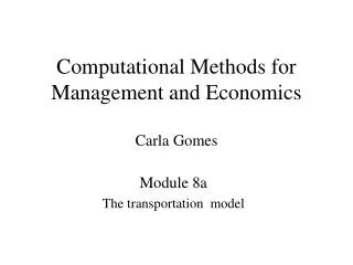
Computational Methods for Management and Economics Carla Gomes. Module 6a Introduction to Simplex (Textbook – Hillier and Lieberman). Algebraic Model for Wyndor Glass Co. Let D = the number of doors to produce W = the number of windows to produce Maximize P = 3 D + 5 W subject to

E N D
Computational Methods forManagement and EconomicsCarla Gomes Module 6a Introduction to Simplex (Textbook – Hillier and Lieberman)
Algebraic Model for Wyndor Glass Co. Let D = the number of doors to produce W = the number of windows to produce Maximize P = 3 D + 5 W subject to D ≤ 4 2W ≤ 12 3D + 2W ≤ 18 and D ≥ 0, W ≥ 0.
Wyndor Glass Edge of Feasible region CPF
LP Concepts • Corner point feasible solution (CPF solution) – intersection of n (or more; n - number of variables) constraint boundaries; • For any LP with n decision variables two CPF solutions are adjacent to each other if they share (n-1) constraint boundaries • Edge of feasible region – intersection of the (n-1) constraint boundaries shared by two adjacent CPF solutions • Optimality test – for any LP problem that possesses at least one optimal solution, if a CPF solution has no adjacent CPF solutions that are better (as measure by Z) then it must be an optimal solution
3D feasible region Edge of feasible region between two CPFS’s the edge is the line that lies at the intersection of the common constraint boundaries of the two CPFS’s
Corner Point Solutions • Corner-point feasible solution – special solution that plays a key role when the simplex method searches for an optimal solution. Relationship between optimal solutions and CPF solutions: • Any LP with feasible solutions and bounded feasible region • (1) the problem must possess CPF solutions and at least one optimal solution • (2) the best CPF solution must be an optimal solution If the problem has exactly one optimal solution it must be a CFP solution If the problem has multiple optimal solutions, at least two must be CPF solutions
Simplex Method Iterative procedure involving the following steps: • Initialization – find initial CPF solution • Optimality test if optimal stop if not optimal go to next iteration • Iteration – find a better CPF solution; go to 2.
Geometric View Point of Simplex Method Iterative procedure involving the following steps: • Initialization – find initial CPF solution Whenever possible pick (0,0) as initial solution • Optimality test – (check value of Z of adjacent CPF solutions) • Iteration – find a better CPF solution; go to 2. • Consider edges that emanate from current CPF solution and pick the one that increases Z at a faster rate • Stop at the first new constraint boundary
Wyndor Glass Let D = the number of doors to produce W = the number of windows to produce Maximize P = 3 D + 5 W Z=30 1 2 Z=36 Edge of Feasible region 3 Z=27 Z=0 0 CPF
Simplex – Key Concepts • Concept 1 – CPF solutions • Simplex methods focuses only on CPF solutions (finite set) • Concept 2 – Flow of simplex method Iterative procedure: • Initialization – find initial CPF solution • Optimality test if optimal stop if not optimal go to next iteration • Iteration – find a better CPF solution; go to 2. • Concept 3– Initialization • Whenever possible pick the origin; otherwise special procedure
Simplex – Key Concepts (cont.) • Concept 4 – Path to optimal solution • Simplex methods always chooses a CPF solution adjacent to the current one • The entire path to the optimal solution is along the edges of the feasible solution • Concept 5 – Choice of new CPF solution • From a CPF solution consider all edges emanating from it but it does not solve for each adjacent CPF solution – it simply identifies the rate of improvement in Z along a given edge and than it picks the one with the largest improvement • Concept 6– Optimality Test • From a given CPF solution check if there is an edge that gives a positive rate of improvement in Z. If not, current CPF is optimal.
s1 0 4 • x1 Setting up Simplex Method for Algebraic Procedure • Algebraic procedure – solving systems of equations converting inequalities into equalities introduction of slack variables • Slack variables • x1 ≤ 4 x1 + s1 = 4 ; s1 = 4 - x1 • x1 ≤ 4 x1 + s1 = 4 and s1 ≥ 0 • Meaning of Slack variables • 0 – the solution lies on the constraint boundary • >0 – solution lies on the feasible region • <0 – solutions lies on the infeasible region • LP Augmented form – standard form + slack variables
Graphical Representation Augmented solution – solution for original variables + slack variables Basic solution augmented corner point solution; Basic feasible solution augmented corner point feasible solution;
Simplex as an algebraic procedure • System of functional constraints n (5) variables (5) and m (3) equations 2 degrees of freedom, (i.e., we can set those two variables to any arbitrary values); they are the nonbasic variables; the other variables are the basic variables; • Simplex chooses to set the non-basic variables to ZERO. • Simplex solves the simultaneous equations to set the values of the basic variables;
Properties of Basic Solutions A basic solution is composed of: • Non-basic variables – • number of non-basic variables equals (total number of variables - number of functional constraints) • They are set to ZERO • Basic variables – • number of basic variables equals number of functional constraints • Their values results from solving the system of functional constraints (non-basic variables set to 0) • They form the Basic Feasible solution – it is a basic solution that satisfies the non-negativity constraints Adjacent basic feasible solutions – all but one of their basic (non-basic) variables are the same moving from one basic feasible solution to an adjacent one involves switching one variable from non-basic to basic and one variable from basic to non-basic (check graph)
Getting ready for the Simplex • Standard form • <= constraints • Non-negativity constraints on all variables • Positive right hand sides (if these assumptions are not valid additional adjustments need to be done) • Transform the objective function and constraints into equalities (introduction of slack variables) What’s wrong with this format? maximize 3x1 + 2x2 - x3 + x4 x1 + 2x2 + x3 - x4 5; -2x1 - 4x2 + x3 + x4 -1; x1 0,x2 0 not equality not equality not equality/negative x3 may be negative
Simplex Procedure • Initialization – origin whenever possible (decision variables 0) (okay if standard form with positive RHS’s; basic feasible solution (BFS): each equation has a basic variable with coefficient 1 (slack variable = RHS) and the variable does not appear in any other eq; the decision variables are the non-basic variables set to 0) • Optimality test – is current BFS optimal? (the coefficients of the objective function of the non-basic variables gives the rate of improvement in Z )
Simplex Procedure (cont.) • Iteration – move to a better adjacent BFS a)Variable entering the basis • Consider non-basic variables (Graphically - Consider edges emanating from current CPF solution) • Pick the variable that increases Z at a faster rate b)Variable leaving the basis • One of the basic variables will become non-basic; write all the basic variables as a function of the entering variable; the most stringent value (i.e., smallest) will be the value for the new entering variable; the basic variable associated with the most stringent constraint will become non-basic, leaving the basis. (Graphically – where to stop? As much as possible without leaving the feasible region) c)Solving for the new BFS • Objective of this step: convert the system of equations into a more convenient form: (1) to perform optimality test and (2) to perform next iteration if necessary • New basic variable should have coefficient 1 in the equation of the leaving variable and 0 in all the other equations, including the objective function; • Valid operations: • Multiplication (or division) of an equation by a non-zero constant • Addition (or subtraction) of a multiple of an equation to (from) another eqution
Simplex Method in Tabular Form • Tabular form – more compact form – it records only the essential information namely: • Coefficients of variables • The constants on the right hand sides • Basic variable in each equation Note: only xj vars are basic and non-basic – we can think of Z as the basic var. of objective function.
Simplex Method in Tabular Form • Assumption: Standard form max; only <= functional constraints; all vars have non-negativity constraints; rhs are positive • Initialization • Introduce slack variables • Decision variables non-basic variables (set to 0) • Slack variables basic variables (set to corresponding rhs) • Transform the objective function and the constraints into equality constraints • Optimality Test • Current solution is optimal iff all the coefficients of objective function are non-negative
Simplex Method in Tabular Form (cont.) • Iteration: Move to a better BFS • Step1 Entering Variable – non-basic variable with the most negative coefficient in the objective function. Mark that column as the pivot column. • Step2 Leaving basic variable – apply the minimum ratio test: • Consider in the pivot column only the coeffcients that are strictly positive • Divide each of theses coefficients into the rhs entry for the same row • Identify the row with the smallest of these ratios • The basic variable for that row is the leaving variable; mark that row as the pivot row; • The number in the intersection of the pivot row with the pivot column is the pivot number
Simplex Method in Tabular Form (cont.) • Iteration: Move to a better BFS • Step3 Solve for the new BFS by using elementary row operations to construct a new simplex tableau in proper form • Divide pivot row by the pivot number • for each row (including objective function) that has a negative coefficient in the pivot column, add to this row the product of the absolute value of this coefficient and the new pivot row. • for each row that has a positive coefficient in the pivot column, add to this row the product the new pivot row.multiplied by the negative of the coefficient.
Wyndor Glass1st Simplex Tableau Optimal? Entering Variable?
What variable will enter the basis? Why? What variable will leave the basis? Why? What transformations do we need to perform to the tableau to get the new basic variable into the right format?
What operations did we perform? 1 – divide the pivot row by 2; 2 – multiplied the new pivot row by (-2) and added it to eq. 3 3 – multiplied the new pivot row by (5) and added it to eq. 0 What are the new basic / non-basic variables?
Optimal? Entering Variable?
What operations did we perform? 1 – divide the pivot row by ; 2 – multiplied the new pivot row by ( ) and added it to eq. 1 3 – multiplied the new pivot row by ( ) and added it to eq. 0 What are the new basic / non-basic variables?