Download
1 / 30
340 likes | 844 Views
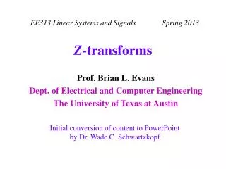
Z Transforms. Another French Mathematician?. Z Transforms. The Z transform is to discrete time systems as the Laplace transform is to continuous time systems. The Fourier transform is the Laplace transform evaluated on the j w axis.

E N D
Z Transforms Another French Mathematician?
Z Transforms The Z transform is to discrete time systems as the Laplace transform is to continuous time systems. The Fourier transform is the Laplace transform evaluated on the jw axis. The discrete Fourier transform is the Z transform evaluated on a unit circle in the Z transform plane.
Z Transforms As with the Laplace and Fourier transforms, the Z transform only if there is a region in the z plane where the Z transform sum converges.
Z Transforms The Z transform is a linear operation: To prove this:
Z Transforms The Z transform also has a time shifting property: This is easily proven: Changing variables:
Z Transforms There is a discrete time unit step function, u(n). This is analogous to the continuous time unit step, u(t): The discrete time unit step is:
Z Transforms We can write a causal signal either this way: Or like this:
Z Transforms Let’s derive some Z transform pairs. First, though, we need several formulas dealing with geometric series. Here’s a finite geometric series: Multiplying both sides by a:
Z Transforms If we subtract the last equation from the preceding one: Solving for SN-1: Note that a can be real, imaginary, or complex, but cannot be equal to 1.
Z Transforms Now consider an infinite geometric series: For this to converge, aN must approach zero as N approaches infinity. In other words, If this condition is met,
Z Transforms if a is complex, it may be written as In which case r < 1 is equivalent to
Z Transforms Now let’s find the Z transform of the discrete time impulse: So Now let’s try the shifted impulse, d(n-k):
Z Transforms Now, let’s take the causal series: This converges if
Z Transforms Using the formula for an infinite geometric series, and substituting cz-1 for a:
Z Transforms Now let’s try this one: Using Euler’s formula:
Z Transforms for c in But we can substitute This gives us:
Z Transforms But this can be rewritten as: And this can be simplified as:
Z Transforms So we have this transform pair: A similar derivation yields this:
Z Transforms Uniqueness “Problem” Recall that this is a transform pair: Now, consider the “anticausal twin” of cnu(n):
Z Transforms This can be rewritten as: So we can derive its Z transform:
Z Transforms But this can also be written as: So: Using the geometric series formula:
Z Transforms We can rearrange this a bit more: But, we already derived this:
Z Transforms The only difference between the Z transform pairs for the causal series and it’s anticausal twin is the region of convergence - so we need to know which series we’re dealing with. Normally it will be the causal one. Examples:
Discrete Time Transfer Function For a continuous time system, the transfer function is: For a continuous time system, the transfer function is:
Discrete Time Transfer Function We have two ways to find the transfer function: 1. Take the Z transforms of the input and output sequences X(z) and Y(z), then divide Y(z) by X(z) 2. Take the Z transform of the system impulse response sequence:
Discrete Time Transfer Function Here’s a difference equation for a generalized discrete time system: Here’s its Z transform, by inspection:
Discrete Time Transfer Function Rearranging, So the transfer function is:
Discrete Time Transfer Function This can also be rewritten as: This is similar to the way we wrote the transfer function of a continuous time system. The lk’s and pk’s are the zeros and poles, respectively.
Discrete Time Transfer Function Since the coefficients (ak and bk) are real numbers, the poles and zeros must either be real, or complex conjugate pairs. Since the feedback coefficients (ak) of an FIR system are all zero, the denominator of its transfer function is 1. Therefore, an FIR system has no poles. It may be referred to as an all-zero system.
Discrete Time Transfer Function Let’s talk about the impulse response for a minute. Suppose we have a discrete-time system with an impulse response h(n), and we drive it with an impulsive input: Then the response is: Or, in the Z transform domain,