Download
1 / 36
360 likes | 445 Views
Topic 2: Production Externalities. Burning Coal. So far we have only considered policies that reduce pollution by reducing output. Indirect way to reduce environmental costs. What if there are ways in which we can make production cleaner? i.e., (E/Q)

E N D
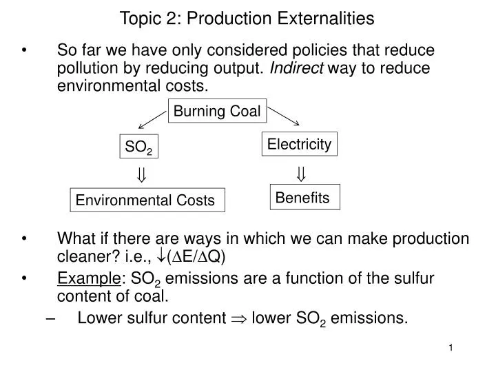
Topic 2: Production Externalities Burning Coal • So far we have only considered policies that reduce pollution by reducing output. Indirect way to reduce environmental costs. • What if there are ways in which we can make production cleaner? i.e., (E/Q) • Example: SO2 emissions are a function of the sulfur content of coal. • Lower sulfur content lower SO2 emissions. Electricity SO2 Benefits Environmental Costs
Topic 2: Production Externalities • In practice, can be many possible levels of sulfur content in coal. • For simplicity, we will assume there are just two types of coal: low sulfur coal and high sulfur coal. • Continuing with coal-fired power plant example… Suppose: • (as before) each ton of SO2 in $300 of damage, irrespective of the level of SO2 emissions (MD = 300); and • each kwh of electricity • 1/10,000th of a ton of SO2 emissions if high sulfur coal; • 1/30,000th of a ton of SO2 emissions if low sulfur coal; High sulfur coal: MECH = $0.03. Low sulfur coal: MECL = $0.01. • Assume initially that price of coal not a function of sulfur content. • MPC not a function of sulfur content Unrealistic: we will relax this assumption later
Topic 2: Production Externalities MSC depending on the sulfur content of coal. If MPC not a function of H or L, then: c MSCH 12 MECH MSCL MSCH = 3 + (1/50)Q A MPC C MSCL = 1 + (1/50)Q B 3 MECL MB 1 Q (thousands kwh) 300 3662/3 1,200 We get the benefit of cleaner production at no cost. Maximized NB = area A if H is used = $13,500 = areas A+B+C if L is used = $20,167 Clearly better to use low sulfur coal
Topic 2: Production Externalities • If L costs the same as H, then clearly efficiency requires that the cleaner input be used. • MSC is lower using L than H. • Will the firm want to use the cleaner input? • Inputs cost the same the firm will be indifferent • No real regulatory problem in ensuring the right choice of input by the firm.
Topic 2: Production Externalities • Problem still remains, however, of getting the firm to produce the right quantity of output, given the use of the clean input. • Even with low sulfur coal, MEC > 0 firm will produce too much output absent government intervention. • So there still is a role for government in ensuring that the firm produces where MSC = MB. • Taxes, quotas, etc, in the output market.
Topic 2: Production Externalities • The more interesting (and realistic) case is where the clean and dirty inputs have different costs. • For instance, it is likely that MPCL > MPCH • Specifically, in our example assume: • MPCH = (1/50)Q; and • MPCL = 1 + (1/50)Q • That is, using low sulfur coal per kwh cost of electricity by 1c.
Topic 2: Production Externalities • Questions: • From the viewpoint of efficiency, do we want H or L? • Will the firm make the right choice of inputs? • If not, what policies will induce the firm to make the right choice? • Once we have induced the right input choice, do we still need government intervention to ensure the right output choice?
Topic 2: Production Externalities • The answers to Qs 1 and 2 are fairly obvious: • From the viewpoint of efficiency, do we want H or L? • Cost of low sulfur coal = 1c extra per kwh produced • Benefit of low sulfur coal = 2c per kwh lower MEC. We want the firm to use low sulfur coal.
Topic 2: Production Externalities • Will the firm make the right choice of inputs? • Cost of low sulfur coal = 1c extra per kwh produced • Benefit to the firm of low sulfur coal = nothing, without some form of government intervention. • the firm doesn’t account for the MEC, so doesn’t care that it is lower using low sulfur coal. Firm will not choose to to use low sulfur coal, absent regulatory inducement. • Can also analyze Qs 1 and 2 graphically.
Topic 2: Production Externalities Low sulfur coal increases production costs by 1c/kwh but reduces MEC by 2c/kwh. MSCH = MPCH + MECH = (1/50)Q + 3 c MSCH MSCL MECL MPCL MPCH MSCL = MPCL + MECL = 1 + (1/50)Q + 1 = 2 + (1/50)Q MECH 3 2 1 Q (thousands kwh) At any level of output, using L rather than H Lower social costs; and Higher private costs L is efficient but not profit- maximizing. Exercise: Calculate the in maximized NB that result from using L rather than H, given the D curve
Topic 2: Production Externalities • How can we induce the firm to adopt the cleaner input? • The policies we have considered so far won’t do it (without modification). • They all target output, not emissions. • Output tax: if we set t = $0.03 per kwh then, including the tax, the firm’s costs are: • MPCH + t = (1/50)Q + 3, if H used • MPCL + t = 1 + (1/50) + 3 = (1/50)Q + 4, if L used H still cheaper for firm than L
Topic 2: Production Externalities • Quota: Mandates a reduction in output, not pollution. • Subsidy on output reduction: Has same effect as tax. • Obvious point is that policy should address the target of interest, which is emissions here (not output).
Topic 2: Production Externalities • BUT, doesn’t mean that we can’t ever achieve efficiency in this context by policies targeting Q. • For example: we could introduce an output tax as follows: • t = $0.03 per kwh for power plants using high sulfur coal; or • t = $0.01 per kwh for power plants using low sulfur coal. • This policy would ensure the firm internalized all EC no matter which input it used. • Would induce all firms choose L rather than H. • Potentially difficult and costly in terms of monitoring/ensuring enforcement. • How do we know whether on any given day a firm is using one type of coal or another?
Topic 2: Production Externalities • Alternative policies to ensure the right input is used: • Require the use of low sulfur coal: • Simply mandate that all firms use the low emissions input. • An example of “command and control” policy. • Tax high sulfur coal: • Note: different from taxing output. • We need to figure out a tax on high sulfur coal that will mean that MPC of producing output is greater for H rather than L. • If H and L are equally productive in terms of electricity output, this simply means making H more expensive than L. • Think about the case where L is less productive.
Topic 2: Production Externalities • Subsidize low sulfur coal: • Similar to the tax on high sulfur coal • We need to figure out a subsidy on L that will mean that MPC of producing output is lower for L rather than H. • So far we have looked at two ways in which emissions of a pollutant can be abated • Pollution abatement = pollution reduction • In the electricity example, abatement can be achieved through: • Reducing output • Switching to a cleaner input.
Topic 2: Production Externalities • In reality pollution can also be reduced through the installation of pollution control equipment. • For instance, SO2 emissions can be reduced through the use of an electro-magnetic precipitator, or “scrubber.” • How does it work? Gaseous SO2 is piped through a “reaction tower.” A slurry of finely ground limestone is also sprayed into the reaction tower. The SO2 reacts with the limestone, 95% of the SO2 is removed and gypsum (CaS04) is formed as a by-product. • Installing equipment such as scrubbers fixed cost for the firm.
Topic 2: Production Externalities • Qualitatively different from other abatement activities/policies we have considered. • per unit output tax • input switching • The decision of whether or not to require the installation of pollution control equipment also introduces a time dimension to the problem. • If we install the equipment, • we incur a (fixed) cost now; and • receive (flow) benefits (in terms of reduced emissions) now and in the future. Both VC (hence shift MC)
Topic 2: Production Externalities • We need some way in which to compare costs today with future benefits. Example: Suppose that • Current emissions = 280 tons of SO2 per year. • Each ton of SO2 $100 of TD (i.e., MD = $100). • Cost of a scrubber = $200,000 • Lifetime of a scrubber = 10 years • Assume (i) VC of scrubber = 0 and (ii) E = 0 if scrubber used.
Topic 2: Production Externalities • Question: Is it economically efficient to install the scrubber? • Tempting to say: • Benefit of scrubber (saved environmental costs) = 10 $28,000 = $280,000 > $200,000 = cost of installing scrubber • Tempting…. But incorrect!! • We can’t compare today’s $s with future $s in this way.
Topic 2: Production Externalities • Dollars today are worth more than the same number of dollars at some time in the future. • This is because if I receive a certain number of dollars today I can invest them more dollars in the future. Example: I have $100 today, which I can invest at 5%. • In 1 year I will have: $100 (1.05) = $105. • In 2 years I will have: $105 (1.05) = ($100 (1.05)) (1.05) = $100 (1.05)2 = $110.25. • In 3 years I will have: $110.25 (1.05) = $100 (1.05)3 = $115.76. Etc…..
Topic 2: Production Externalities General formula: FV of a single payment of X in n years time = X(1+r)n. = 100(1+r) = 100(1+r)2 • Tells us about future value (FV) of $100. If the interest rate is 5%, the FV of $100 is: • $105 in one year • $110.25 in two years • $115.76 in three years • FV tells how much a certain amount of today’s money will be worth at some point in the future. • In this class, we will more often be interested in the present value (PV) of a sum of money. • PV tells us how much a certain amount of future money is worth today. • For instance, if installing a scrubber will generate an annual benefit of $28,000 ten years from now, what is that worth to us now? = 100(1+r)3
Topic 2: Production Externalities Example: • Suppose r = 5%. What is $105 received in one year’s time worth to us now? • i.e., what is the PV of $105 in 1 years time? • We already know that if we invest $100 at 5%, then we will have $105 in one year. having $100 now and $105 in one year are (in some sense) equivalent. the PV of $105 in one years time is $100.
Topic 2: Production Externalities • Similar logic the PV of $110.25 in 2 years time is $100. etc. • General formula: • PV of a single payment of X in n years time = X/(1+r)n. • Often useful to think of PV as the amount of money you would need to invest now, in order to have X in n years.
Topic 2: Production Externalities Note timing assumption here! • General PV formula can help us figure out the PV of the saved EC from installing scrubber. (assume in this ex that r = 5%) • Savings of $28,000 per year for 10 years. • Saved EC in the: • 1st year: PV = 28,000/1.05 = $26,666.67 • 2nd year: PV = 28,000/(1.05)2 = $25,396.83 …… • 10th year: PV = 28,000/(1.05)10 = $17,189.57 • Total PV of saved EC (= benefit of installing scrubber) = $26,666.67 + $25,396.83 + … + $17,189.57 = $216,298.58 < 10 $28,000 • Fixed cost of installing scrubber = $200,000 • Benefit of scrubber exceeds cost efficient to install.
Topic 2: Production Externalities The effect of discounting graphically: (finding the PV referred to as “discounting”) annual savings in EC PV of EC savings r = 5% Saving to EC that occur in ten years time are worth much less (measured in PV dollars) than savings to EC in one year.
Higher interest rates lower PV: Topic 2: Production Externalities r = 5% r = 10% Using a higher r discounting the future more placing less weight on the future. If r = 10% in this example, the PV of benefits from installing scrubber = $172,047.88 If correct to use r = 10%, then NOT efficient to install scrubber.
Topic 2: Production Externalities • Using the general PV formula can be computationally inefficient if we are looking at long time horizons. • For instance, if the scrubber lasted for 50 years, or longer. • If the scrubber lasted forever, this is easy computationally. • Formula for the PV of an infinite stream of payments of X per year (beginning in 1 years time) at interest rate r: • PV = X/r
Topic 2: Production Externalities • Example: What is the PV of $100 per year forever, beginning in one year, if r = 10%? • PV = $100/(0.10) = $1,000 • Intuition for formula? Suppose we took $1,000 invested at 10%. • After 1st year, interest income = $100. Can withdraw that, leaving the principal intact at $1,000. • After 2nd year, interest income = $100. Can withdraw that, leaving the principal intact at $1,000. • After 3rd year, interest income = $100. Can withdraw that, leaving the principal intact at $1,000. • And so on….
Topic 2: Production Externalities • Tells us that - if r = 10% - having $1,000 now, is the same as having an income stream of $100 per year forever. • We can combine the • formula for the PV of 1 payment received in n years time • PV = X/(1+r)n; with • the formula for the PV of an infinite stream of payments • PV = X/r To solve the problem of finding the PV of a finite stream of payments that lasts for a large number of periods.
Topic 2: Production Externalities • Suppose the scrubber has a lifetime of 50 years, and in each year it operates it reduced EC by $28,000. Still assume r = 5%. • This is a finite stream of benefits, which we can actually think of as being the difference between two infinite streams of benefits. PV of finite stream = PV of A - PV of B $28,000 Stream A Stream B years 0 1 2 3 …………. 50 51 52 53 …………………… ∞ Infinite stream A: $28,000 per year forever, beginning in year 1. Infinite stream B: $28,000 per year forever, beginning in year 51. PV of finite stream of $28,000 per year beginning in year 1 = PV of infinite stream A - PV of infinite stream B.
Topic 2: Production Externalities Infinite stream A: $28,000 per year forever, beginning in year 1. • PV = $28,000/0.05 = $560,000 Infinite stream B: $28,000 per year forever, beginning in year51. • PV in year50 = $28,000/0.05 = $560,000. $28,000 Stream A Stream B years 0 1 2 3 …………. 50 51 52 53 …………………… ∞ PV of stream B at year 50 = $560,000 PV of stream A at year 0 = $560,000 Infinite stream B is worth $560,000 to us in year50 dollars.
Topic 2: Production Externalities Infinite stream B: worth $560,000 to us in year50 dollars. • What is this worth to us now (in year0 dollars)? • PV of $560,000 received in 50 years = $560,000/(1.05)50 = $48,834.09. $28,000 Stream A Stream B years 0 1 2 3 …………. 50 51 52 53 …………………… ∞ PV of stream B at year 50 = $560,000 PV of stream A at year 0 = $560,000 PV of stream B at year 0 = $48,834.09
Topic 2: Production Externalities • Recall: we are trying to find the PV of $28,000 of benefits received every year for 50 years. • PV of the 50 year stream = PV of stream A - PV of stream B. = $560,000 - $48,834.09 = $511,165,91 $28,000 Stream A Stream B years 0 1 2 3 …………. 50 51 52 53 …………………… ∞ Tell us that the PV of the saved environmental costs = $511,165.91, over the 50 year life of the pollution control equipment. PV of stream A at year 0 = $560,000 - PV of stream B at year 0 = $48,834.09
Topic 2: Production Externalities • PV of benefits from activities such as installing pollution control equipment yield a maximum willingness to pay for this equipment (if efficiency is our criterion for decision-making). • Recall in example the cost of the scrubber was $200,000. • We have seen that, if the scrubber EC by $28,000 per year for 50 years, the PV of benefits is $511,165.91. • Tells us that the PV of net benefits associated with installing the scrubber = present value TB - TC = $511,165.91 - $200,000 = $311,165.91
Topic 2: Production Externalities • Net benefits in this context often referred to as the Net Present Value (NPV). • NPV = PV of Total Benefits - PV of Total Costs. • Note: in example, the costs were incurred today, so no need to find the PV of costs (not always the case). • Efficiency in a dynamic context: • A context in which benefits and costs fall at different times. • Maximizing NB maximizing NPV.
Topic 2: Production Externalities • Decision rules for dynamic choices: • Binary decision-making: Do we undertake a given project? • Example: do we install a scrubber or not? • Yes, if the NPV is positive. • More complex choice: If we are faced with a number of different projects, which (if any) do we undertake? • Example: if there is a choice among different pollution control technologies, which should we adopt? • Undertake the project with the highest NPV.