Download
1 / 62
620 likes | 622 Views
This article explores the fundamentals and optimization techniques for stencil computations on CPUs. Topics include spatial, sequential, and temporal locality, arithmetic intensity, and performance models. Case studies on 7-point and 27-point stencils, lattice Boltzmann methods, and high-order wave equations are discussed.

E N D
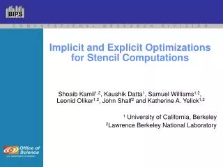
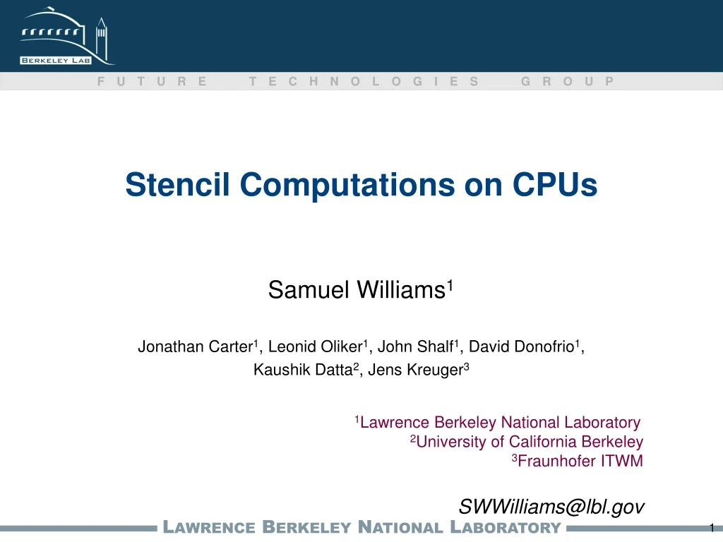
Stencil Computations on CPUs Samuel Williams1 Jonathan Carter1, Leonid Oliker1, John Shalf1, David Donofrio1, Kaushik Datta2, Jens Kreuger3 • 1Lawrence Berkeley National Laboratory 2University of California Berkeley3Fraunhofer ITWM SWWilliams@lbl.gov
Outline Fundamentals Roofline Performance Model Optimization of 7- and 27-point Stencils Optimization of Lattice Boltzmann Methods Optimization of High-order Wave Equations Summary
Three Classes of Locality • Spatial Locality • data is transferred from cache to registers in words. • However, data is transferred to the cache in 64-128Byte lines • using every word in a line maximizes spatial locality. • transform data structures into structure of arrays (SoA) layout • Sequential Locality • Many memory address patterns access cache lines sequentially. • CPU’s hardware stream prefetchers exploit this observation to hide speculatively load data to memory latency. • Transform loops to generate (a few) long, unit-stride accesses. • Temporal Locality • reusing data (either registers or cache lines) multiple times • amortizes the impact of limited bandwidth. • transform loops or algorithms to maximize reuse.
Arithmetic Intensity • True Arithmetic Intensity (AI) ~ Total Flops / Total DRAM Bytes • Some HPC kernels have an arithmetic intensity that scales with problem size (increased temporal locality) • Others have constant intensity • Arithmetic intensity is ultimately limited by compulsory traffic • Arithmetic intensity is diminished by conflict or capacity misses. O( log(N) ) O( 1 ) O( N ) A r i t h m e t i c I n t e n s i t y SpMV, BLAS1,2 FFTs Stencils (PDEs) Dense Linear Algebra (BLAS3) Lattice Methods Particle Methods
Roofline Model 256.0 128.0 64.0 32.0 16.0 8.0 4.0 2.0 1.0 0.5 1/8 1/4 1/2 1 2 4 8 16 • Visualizes how bandwidth, compute, locality, and optimization bound performance. • Based on application characteristics, one can infer what needs to be done to improve performance. Opteron 2356 (Barcelona) peak DP mul / add imbalance attainable GFLOP/s w/out SIMD Stream Bandwidth w/out SW prefetch w/out NUMA +conflict miss traffic +capacity miss traffic +write allocation traffic only compulsory miss traffic w/out ILP actual FLOP:Byte ratio
PDEs on Structured Grids:7- and 27-point Stencils K. Datta, M. Murphy, V. Volkov, S. Williams, J. Carter, L. Oliker, D. Patterson, J. Shalf, K. Yelick, "Stencil Computation Optimization and Autotuning on State-of-the-Art Multicore Architectures", Supercomputing (SC), 2008. K. Datta, S. Williams, V. Volkov, J. Carter, L. Oliker, J. Shalf, K. Yelick, "Auto-tuning the 27-point Stencil for Multicore", The Fourth International Workshop on Automatic Performance Tuning (iWAPT 2009), Tokyo, Japan, October 1-2, 2009. K. Datta, S. Williams, V. Volkov, J. Carter, L. Oliker, J. Shalf, K. Yelick, "Auto-tuning Stencil Computations on Diverse Multicore Architectures", Scientific Computing on Multicore and Accelerators, edited by: JakubKurzak, David A. Bader, Jack Dongarra, CRC Press, 2010, ISBN: 978-1-4398253-6-5.
7-point Stencil z+1 +Z y-1 x+1 x,y,z x-1 y+1 +Y z-1 +X PDE grid stencil for heat equation PDE • Simplest derivation of the Laplacian operator results in a constant coefficient 7-point stencil for all x,y,z: u(x,y,z,t+1) = alpha*u(x,y,z,t) + beta*( u(x,y,z-1,t) + u(x,y-1,z,t) + u(x-1,y,z,t) + u(x+1,y,z,t) + u(x,y+1,z,t) + u(x,y,z+1,t) ) • Clearly each stencil performs: • 8 floating-point operations • 8 memory references all but 2 should be filtered by an ideal cache • 6 memory streams all but 2 should be filtered (less than # HW prefetchers)
Stencil Performance(reference code, double-precision, 2563, single node) • NOTE (for 7-point): 1 GStencil/s = 8 Gflop/s • No scalability • Poor performance • VF performance peaks using ½ of one socket Reference Implementation
Data Structure Transformations + = • Caches have limited associativity • padding arrays avoids cache conflict misses • Explore paddings up to 32 in unit stride NUMA SMPs are common. one malloc() with parallel initialization (exploit first touch)
Code Transformations (1) • Naïve parallelization gives each thread Z/P • Cache blocking gives each thread a number of consecutive (CX × CY × CZ) blocks. • avoids LLC capacity misses • Explore all possible power of 2 blockings 3 3 3 3 2 3 3 Thread 3 2 3 3 1 2 1 2 3 1 2 0 2 2 Thread 2 1 2 3 3 0 1 1 2 3 2 0 0 Thread 1 1 0 1 1 3 2 1 0 1 2 1 0 2 0 Thread 0 0 1 0 0 0 0 Register Blocking (3D unroll and jam) attempts to create locality in the register file/L1 cache Many possible blockings (RX × RY × RZ) maximizes ILP, minimizes L1 BW Explore all possible power of 2 blockings
Code Transformations (2) SW Prefetching supplements HW prefetchers and hides memory latency Explore a number of prefetch distances Thread blocking adds a second level of parallelization for SMT architectures. inter-thread locality via shared L1’s Explicit SIMDizationattempts to compensate for a compiler’s inability to generate good SIMD code. Cache bypass exploits instructions designed to eliminate write allocate traffic
Auto-tuning We’ve enumerated an enormous orthogonal optimization space. To explore it, we implemented an auto-tuner that is capable of generating a series of parameterized (e.g. cache block size) code variants (e.g. register block size) and efficiently explore them The result is a degree of performance portability across a wide range of architectures
Auto-tuned Stencil Performance(full tuning, double-precision, 2563, single node) • Dramatically better performance and scalability • Clearly cache blocking (capacity misses) were critical to performance despite these machines having 8-16MB of cache • XLC utterly failed to register block (unroll&jam) • Array padding was critical on VF (conflict misses) +2nd pass thru greedy search +Cache bypass +Explicit SIMDization +Thread Blocking +SW Prefetching +Register Blocking +Cache Blocking +Padding +NUMA Reference Implementation
Roofline Model 256.0 128.0 64.0 32.0 16.0 8.0 4.0 2.0 1.0 0.5 1/8 1/4 1/2 1 2 4 8 16 • Where are we on the roofline? • 1.95 gstencil/s • = 15.6 gflop/s • flop:byte < 0.5 (movntpd) Xeon X5550 (Nehalem) peak DP mul / add imbalance Stream Bandwidth w/out SIMD attainable GFLOP/s w/out NUMA only compulsory miss traffic w/out ILP actual FLOP:Byte ratio
27-point stencil • Here, we have: • 4 coefficients • 30 flop’s • higher register pressure/reuse • arithmetic intensity of up to 1.875 flops/byte
Algorithmic Transformations • Subtly performance (stencils/s) can go down (more flops per stencil) but both performance (gflop/s) and time to solution can improve (fewer sweeps to converge) • Two approaches: • 27-point stencil (~30 flops per stencil) • 27-point stencil with inter-stencil common subexpression elimination (~20+ flops/stencil)
Auto-tuned 27-point Stencil (full tuning, double-precision, 2563, single node) • When embedded in an iterative solver, 27-point should require fewer iterations to converge • However, performance (stencils/second) is lower, so one must tune for the right balance of performance per iteration and number of iterations • Observe Clovertown performance didn’t change (bandwidth is so poor it’s the bottleneck in either case) +Common Subexpression Elimination +Cache bypass
27-point on Cell and GPU’s(full tuning, double-precision, 2563, single node) All the stencil work was also implemented via an auto-tuner on a QS22 CBE, and a direct optimized implementation on a GTX280. Clearly, Cell is bandwidth-starved
Lattice Boltzmann Methods:LBMHD Samuel Williams, Jonathan Carter, Leonid Oliker, John Shalf, Katherine Yelick, "Extracting Ultra-Scale Lattice Boltzmann Performance via Hierarchical and Distributed Auto-Tuning", Supercomputing (SC), 2011. Samuel Williams, Jonathan Carter, Leonid Oliker, John Shalf, Katherine Yelick, "Lattice Boltzmann Simulation Optimization on Leading Multicore Platforms", International Parallel & Distributed Processing Symposium (IPDPS), 2008. Best Paper, Applications Track
25 LBMHD 12 0 23 12 4 25 26 15 15 14 6 2 22 14 8 23 18 18 21 26 24 21 10 9 20 20 22 13 1 13 11 5 24 17 17 16 7 3 16 19 19 +Z +Z +Z +Y +Y +Y +X +X +X macroscopic variables momentum distribution magnetic distribution • Lattice Boltzmann Magnetohydrodynamics (CFD+Maxwell’s Equations) • Plasma turbulence simulation via Lattice Boltzmann Method for simulating astrophysical phenomena and fusion devices • Three macroscopic quantities: • Density • Momentum (vector) • Magnetic Field (vector) • Two distributions: • momentum distribution (27 scalar components) • magnetic distribution (15 Cartesian vector components)
LBMHD • Code Structure • time evolution through a series of collision( ) and stream( ) functions • stream( ) • performs a ghost zone exchange of data to facilitate distributed memory implementations as well as boundary conditions • should constitute 10% of the runtime • collision( )’sArithmetic Intensity: • Must read 73 doubles, and update 79 doubles per lattice update (1216 bytes) • Requires about 1300 floating point operations per lattice update • Just over 1.0 flops/byte (ideal architecture) • Suggests LBMHD ismemory-boundon the Cray XT4/XE6. • Structure-of-arrays layout (component’s are separated) ensures that cache capacity requirements are independent of problem size • However, TLB capacity & streams increases to >150 entries • periodic boundary conditions
LBMHD Stencil Simplified example reading from 9 arrays and writing to 9 arrays Actual LBMHD reads 73, writes 79 arrays
Vectorization • Two phases with a lattice method’s collision() operator: • reconstruction of macroscopic variables • updating discretized velocities • Nominally, all flops are completed for one point before proceeding to the next. • Change to do a vector’s worth one operation at a time • Regularizes memory access pattern at the expense of increased L1 bandwidth.
Results Explored performance on 3 ultrascale machines using 2048 nodes on each and running a 1GB, 4GB, and if possible 16GB(per node) problem size. IBM Blue Gene/P at Argonne (Intrepid) 8,192 cores Cray XT4 at NERSC (Franklin) 8,192 cores Cray XE6 at NERSC (Hopper) 49,152 cores
Performance Results(using 2048 nodes on each machine) 1P Quad-core Opteron Blue Gene/P 2P 12-core Opteron We present the best data for progressively more aggressive auto-tuning efforts Remember, Hopper has 6x as many cores per node as Intrepid or Franklin. So performance per node is far greater. auto-tuning can improve performance ISA-specific optimizations (e.g. SIMD intrinsics) help more Overall, we see speedups of up to 3.4x As problem size increased, so to does performance. However, the value of threading is diminished.
Performance Results(using 2048 nodes on each machine) We present the best data for progressively more aggressive auto-tuning efforts Remember, Hopper has 6x as many cores per node as Intrepid or Franklin. So performance per node is far greater. auto-tuning can improve performance ISA-specific optimizations (e.g. SIMD intrinsics) help more As problem size increased, so to does performance. However, the value of threading is diminished. For small problems, MPI time can dominate runtime on Hopper Threading mitigates this
Performance Results(using 2048 nodes on each machine) We present the best data for progressively more aggressive auto-tuning efforts Remember, Hopper has 6x as many cores per node as Intrepid or Franklin. So performance per node is far greater. auto-tuning can improve performance ISA-specific optimizations (e.g. SIMD intrinsics) help more As problem size increased, so to does performance. However, the value of threading is diminished. For large problems, MPI time remains a small fraction of overall time
Energy Results(using 2048 nodes on each machine) Ultimately, energy is becoming the great equalizer among machines. Hoper has 6x the cores, but burns 15x the power of Intrepid. To visualize this, we explore energy efficiency (Mflop/s per Watt) Clearly, despite the performance differences, energy efficiency is remarkably similar.
PDEs on Structured Grids:High-order Wave Equation Stencils J. Kreuger, D. Donofrio, J. Shalf, M. Mohiyuddin, S. Williams, L. Oliker, F.J. Pfreundt, "Hardware/Software Co-design for Energy-Efficient Seismic Modeling", (to appear at) Supercomputing (SC), 2011.
8th Order Wave Equation(25-point stencil) z+4 +Z z+3 z+2 y-4 y-3 z+1 y-2 x+1 y-1 x+1 x,y,z x+1 x+1 x-1 x-2 y+1 x-3 y+2 x-4 +Y z-1 y+3 y+4 z-2 +X z-3 PDE grid stencil for wave equation PDE z-4 • 8th Order Finite Difference isotropic, inhomogeneous wave equation: for all x,y,z: laplacian = coeff[0]*u[x,y,z,t]; for(r=1;r<=4;r++){ laplacian += coeff[r]*( u[x,y,z+r,t] + u[x,y,z-r,t] + u[x,y+r,z,t] + u[x,y-r,z,t] + u[x+r,y,z,t] + u[x-r,y,z,t] ); } u[x,y,z,t+1] = 2.0*u[x,y,z,t] - u[x,y,z,t-1] + vel[x,y,z,t]*laplacian; • Clearly each 8th order wave equation stencil performs: • 33 floating-point operations • 29 memory references all but 4 should be filtered by an ideal cache • 20 memory streams all but 4 should be filtered
Comparisons:High-order Wave Eqn. vs. LBMHD/7/27pt • Compared to the 7-pt/27-point stencil, high-order wave equation: • generates far more address streams • access 4 arrays instead of 2 • demands a much larger cache working set • However, compared to LBMHD, high-order wave equation: • performs far fewer flops • generates far fewer streams • has temporal reuse (LBMHD has no temporal reuse) and thus demands a much larger cache working set. • With proper optimization, based on the Roofline model, we expect all three to be memory bound.
Reference Performance(single node, single-precision, 5123) start with reference implementation on a 2P Nehalem-based Xeon Fermi-accelerated node is 17x faster This is surprising given Fermi only less than 3x the sustained bandwidth as this 2P Nehalem NOTE: no MPI communication
Roofline Model 512.0 256.0 128.0 64.0 32.0 16.0 8.0 4.0 2.0 1.0 1/8 1/4 1/2 1 2 4 8 16 • Where are we on the roofline? • 255 mstencil/s = 8.4 gflop/s • flop:byte << 1.65 • compulsory misses & • write allocates Xeon E5530 (Nehalem) peak SP mul / add imbalance attainable GFLOP/s Stream Bandwidth w/out SIMD w/out NUMA write allocate arithmetic intensity w/out ILP actual FLOP:Byte ratio
Optimizations • Roofline limit is about 1800 mstencil/s • To improve CPU performance we can apply the set of optimizations explored for the 7- and 27-point stencils including: • Loop unrolling / register blocking • Cache Blocking - we parallelize in Y(cores) and Z (sockets) • Explicit SIMDization • NUMA • Pipelining (shifting) data through SIMD registers to reduce L1 bandwidth • Cache Bypass (non-temporal stores)
Optimized Performance(single node, single-precision, 5123) Optimizations improved CPU performance by about 5x Some CPU performance has been left on the table GPUs remained 3-4x faster per node MPI communication will mitigate the GPU performance advantage
Energy Efficiency Power and Energy are becoming an increasing constraint on supercomputer scale and cost. Although the Fermi-accelerated node delivers over 3x better performance, it requires 33% more sustained power (and 66% more peak power) Nevertheless, GPUs still offer a 2-3x energy efficiency advantage over current Intel CPUs (ignoring inter-node communication)
Vectorization and AVX We can leverage the vectorizationtechnique from LBMHD to improve the 12th order performance to over 1000 mstencil/s (+20%) However, performance on the 8th order remained the same. This suggests there is a richer tuning space worthy of additional future exploration. Additionally, Intel’s latest Sandy Bridge supports 256bit SIMD (AVX) Unfortunately, the STREAM bandwidth per socket is about the same as the current Nehalem processors. As such, Sandy Bridge’s sustained performance (as well as energy efficiency) on memory-bound high-order wave equations remained roughly the same as Nehalem.
CoDEx and Green Wave J. Kreuger, D. Donofrio, J. Shalf, M. Mohiyuddin, S. Williams, L. Oliker, F.J. Pfreundt, "Hardware/Software Co-design for Energy-Efficient Seismic Modeling", (to appear at ) Supercomputing (SC), 2011.
Co-Design for Exascale (CoDEx) • CoDEx (Co-Design for Exascale) is collaborative project at LBNL/LLNL/SNL aimed at creating a HW/SW co-design methodology for maximizing the energy efficiency of exascale systems • Based on manycore architecture that integrates the parameterizableTensilicaXTensa embedded core • Couples: • SW and FPGA-based processor simulators (Tensilica and RAMP) • SW network simulators (SST) • HW design tools, • SW analysis tools (ROSE) • Auto-tuners, • etc.. Into a single design methodology designed to extract maximum energy efficiency on specific classes of applications • Its first use was in the context of Climate Computing where it was used to design the Green Flash processor.
Green Wave Design • In the context of seismic modeling • Intel’s commodity CPUs are burdened by backwards compatibility and a focus on consumer apps. • Substantial energy overhead per flop (and per byte of DRAM BW) • GPU’s are focused on performance/node rather than energy efficiency • In collaboration with ITWM, we examined leveraging our CoDEx tool suite for seismic modeling. • The result is what we call Green Wave: • 128 TensilicaXTensa cores (scalar FMA) running at 1GHz • 8KB L1 + 256KB Local Store per core. • cached loads/stores for small accesses • DMA’s for block transfers • 4xDDR3-1600 memory controllers => 50GB/s of memory bandwidth • customized instructions for stencil address calculations • <300mm2 and <70W at 45nm
Green Wave Performance Performance per socket is better than Nehalem, but lower than Fermi
Green Wave Efficiency However, as power per node is lower than either Fermi or Nehalem, Energy efficiency is far superior (up to 3x better than Fermi). Half of Green Wave’s power is in the memory subsystem (where it should be for memory-bound computations)
Summary We’ve shown that CPU performance optimization and auto-tuning can greatly improve performance on a variety of stencil codes. In order to deal with the conventional on-chip memory hierarchy (registers, L1, L2, L3…) in conjunction with HW prefetchers, we must carefully balance loop unrolling, cache blocking, and auxiliary arrays. Although GPU’s deliver better performance and efficiency than CPUs, the gap is closing and potential GPU speedup is increasingly limited by finite bandwidth and inter-node communication time. To resolve this, we present a HW/SW co-designed solution named “Green Wave” that maximizes energy efficiency for the isotropic, inhomogeneous, high-order wave equations seen in seismic codes.
Questions? Acknowledgments Research supported by DOE Office of Science under contract number DE-AC02-05CH11231. All XT4/XE6 simulations were performed on the XT4 (Franklin) and XE6 (Hopper) at the National Energy Research Scientific Computing Center (NERSC). This research used resources of the Argonne Leadership Computing Facility at Argonne National Laboratory, which is supported by the Office of Science of the U.S. Department of Energy under contract DE-AC02-06CH11357. 2005. George Vahala and his research group provided the original (FORTRAN) version of the LBMHD code. Jonathan Carter provided the optimized (FORTRAN) implementation that served as a basis for the LBMHD portion of this talk.
Roofline ModelBasic Concept Attainable Performanceij = min FLOP/s with Optimizations1-i AI * Bandwidth with Optimizations1-j • Synthesize communication, computation, and locality into a single visually-intuitive performance figure using bound and bottleneck analysis. • whereoptimization i can be SIMDize, or unroll, or SW prefetch, … • Given a kernel’s arithmetic intensity (based on DRAM traffic after being filtered by the cache), programmers can inspect the figure, and bound performance. • Moreover, provides insights as to which optimizations will potentially be beneficial.
Roofline ModelBasic Concept 256.0 128.0 64.0 32.0 16.0 8.0 4.0 2.0 1.0 0.5 1/8 1/4 1/2 1 2 4 8 16 • Plot on log-log scale • Given AI, we can easily bound performance • But architectures are much more complicated • We will bound performance as we eliminate specific forms of in-core parallelism Opteron 2356 (Barcelona) peak DP attainable GFLOP/s Stream Bandwidth actual FLOP:Byte ratio