Download
1 / 16
160 likes | 164 Views
Hands-On Session: Regression Analysis. What we have learned so far Use data viewer ‘afni’ interactively Model HRF with a shape-prefixed basis function Assume the brain responds with the same shape in any active regions regardless stimulus types

E N D
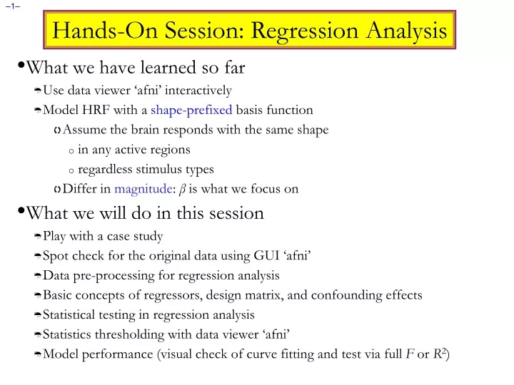
Hands-On Session: Regression Analysis • What we have learned so far • Use data viewer ‘afni’ interactively • Model HRF with a shape-prefixed basis function • Assume the brain responds with the same shape • in any active regions • regardless stimulus types • Differ in magnitude: β is what we focus on • What we will do in this session • Play with a case study • Spot check for the original data using GUI ‘afni’ • Data pre-processing for regression analysis • Basic concepts of regressors, design matrix, and confounding effects • Statistical testing in regression analysis • Statistics thresholding with data viewer ‘afni’ • Model performance (visual check of curve fitting and test via full F or R2)
Preparing Data for Analysis • Six preparatory steps are common: • Temporal alignment (sequential/interleaved): 3dTshift • Image registration (aka realignment): 3dvolreg • Spatial normalization (standard space conversion): adwarp, @auto_tlrc, anlign_epi_anat.py • Blurring: 3dmerge, 3dBlurToFWHM, 3dBlurInMask • Masking: 3dAutomask or 3dClipLevel • Conversion to percentile: 3dTstat and 3dcalc • Censoring out time points that are bad: 3dToutcount (or 3dTqual) and 3dvolreg • Not all steps are necessary or desirable in any given case
A Case Study • The Experiment • Cognitive Task: Subjects see photographs of two people interacting • Mode of communication - 3 categories: telephone, email, or face-to-face. • Affect: negative, positive, or neutral in nature. • Experimental Design: 3x3 Factorial design, BLOCKED trials • Factor A: CATEGORY - (1) Telephone, (2) E-mail, (3) Face-to-Face • Factor B: AFFECT - (1) Negative, (2) Positive, (3) Neutral • A random 30-second block of photographs for a task (ON), followed by a 30-second block of the control condition of scrambled photographs (OFF)... • Each run has 3 ON blocks, 3 OFF blocks. 9 runs in a scanning session.
Illustration of Stimulus Conditions AFFECT Negative Positive Neutral “You are the best project leader!” “Your project is lame, just like you!” “You finished the project.” Telephone CATEGORY "Your new haircut looks awesome!" "Ugh, your hair is hideous!" "You got a haircut." E-mail “I curse the day I met you!” “I feel lucky to have you in my life.” “I know who you are.” Face-to-Face • Data Collected • 1 Anatomical (MPRAGE) dataset for each subject • 124 axial slices • voxel dimensions = 0.938 x 0.938 x 1.2 mm • 9 runs of Time Series (EPI) datasets for each subject • 34 axial slices x 67 volumes (TRs) = 2278 slices per run • TR = 3 sec; voxel dimensions = 3.75 x 3.75 x 3.5 mm • Sample size, n=16 (all right handed)
Multiple Stimulus Classes • Summary of the experiment • 9 related communication stimulus types in a 3x3 design of Category by Affect (stimuli are shown to subject as pictures) • Telephone, Email & Face-to-face = categories • Negative, Positive & Neutral = affects • telephone stimuli: tneg, tpos, tneu • email stimuli: eneg, epos, eneu • face-to-face stimuli: fneg, fpos, fneu • Each stimulus type has 3 presentation blocks of 30 s duration • Scrambled pictures (baseline) are shown between blocks • 9 imaging runs, 64 useful time points in each • Originally, 67 TRs per run, but skip first 3 for MRI signal to reach steady state (i.e., eliminate initial transient spike in data) • So 576 TRs of data, in total (649) • Registered (3dvolreg) dataset: rall_vr+orig • Slice timing is not important in this case
Regression with Multiple Model Files • linear trend • try to use 2 CPUs • run start indexes • stimulus times • '|' indicates new run • response model 3dDeconvolve -input rall_vr+orig –polort 2 \ -jobs 2 \ -concat '1D: 0 64 128 192 256 320 384 448 512' \ -num_stimts 15 -local_times \ -stim_times 1 '1D: 0 | | | 120 | | | | | 60' 'BLOCK(30)' \ -stim_label 1 tneg \ -stim_times 2 '1D: * | | 120 | | 0 | | | | 120' 'BLOCK(30)' \ -stim_label 2 tpos \ -stim_times 3 '1D: * | 120 | | 60 | | | | | 0' 'BLOCK(30)' \ -stim_label 3 tneu \ -stim_times 4 '1D: 60 | | | | | 120 | 0 | |' 'BLOCK(30)' \ -stim_label 4 eneg \ -stim_times 5 '1D: * | 60 | | 0 | | | 120 | |' 'BLOCK(30)' \ -stim_label 5 epos \ -stim_times 6 '1D: * | | 0 | | 60 | | | 60 |' 'BLOCK(30)' \ -stim_label 6 eneu \ -stim_times 7 '1D: * | 0 | | | 120 | | 60 | |' 'BLOCK(30)' \ -stim_label 7 fneg \ -stim_times 8 '1D: 120 | | | | | 60 | | 0 |' 'BLOCK(30)' \ -stim_label 8 fpos \ -stim_times 9 '1D: * | | 60 | | | 0 | | 120 |' 'BLOCK(30)' \ -stim_label 9 fneu \ • Script file rall_decon does the job: • Run this script by typing tcsh rall_regress (takes a few minutes) • stimulus label continued…
Regression with Multiple Model Files (continued) • motion regressor • apply to baseline -stim_file 10 motion.1D'[0]' -stim_base 10 \ -stim_file 11 motion.1D'[1]' -stim_base 11 \ -stim_file 12 motion.1D'[2]' -stim_base 12 \ -stim_file 13 motion.1D'[3]' -stim_base 13 \ -stim_file 14 motion.1D'[4]' -stim_base 14 \ -stim_file 15 motion.1D'[5]' -stim_base 15 \ -gltsym 'SYM: tpos -epos' -glt_label 1 TPvsEP \ -gltsym 'SYM: tpos -tneg' -glt_label 2 TPvsTNg \ -gltsym 'SYM: tpos tneu tneg -epos -eneu -eneg' \ -glt_label 3 TvsE \ -fout -tout \ -bucket rall_func -fitts rall_fitts \ -xjpeg rall_xmat.jpg -x1D rall_xmat.x1D • symbolic GLT • label the GLT • statistic types to output • 9 visual stimulus classes were given using -stim_times • important to include motion parameters as regressors? • this would remove the confounding effects due to motion artifacts • 6 motion parameters as covariates via -stim_file and -stim_base • motion.1D was generated from 3dvolreg with the -1Dfile option • we can test the significance of the inclusion with –gltsym • Switch from -stim_base to -stim_label roll … • Use -gltsym 'SYM: roll \ pitch \yaw \dS \dL \dP'
} } Regressor Matrix for This Script (via -xjpeg) } Visual stimuli Baseline Motion • 18 baseline regressors • linear baseline • 9 runs times 2 params • 9 visual stimulus regressors • 33 design • 6 motion regressors • 3 rotations and 3 shifts aiv rall_xmat.jpg
Regressor Matrix for This Script (via -x1D) baseline regressors: via 1dplot -sepscl rall_xmat.x1D'[0..17]'
Regressor Matrix for This Script(via -x1D) • motion regressors • visual stimuli 1dplot -sepscl rall_xmat.x1D'[18..$]'
Options in 3dDeconvolve - 1 -concat '1D: 0 64 128 192 256 320 384 448 512' • “File” that indicates where distinct imaging runs start inside the input file • Numbers are the time indexes inside the dataset file for start of runs • In this case, a text format .1D file put directly on the command line • Could also be a filename, if you want to store that data externally -num_stimts 15 -local_times • We have 9 visual stimuli (+6 motion), so will need 9 -stim_times below • Times given in the -stim_times files are local to the start of each run (vs. -global_times meaning times are relative the start of the first run) -stim_times 1 '1D: 0.0 | | | 120.0 | | | | | 60.0' 'BLOCK(30)' • “File” with 8 lines, each line specifying the start time in seconds for the stimuli within the corresponding imaging run, with the time measured relative to the start of the imaging run itself (local time)
Options in 3dDeconvolve - 2 -gltsym 'SYM: tpos -epos' -glt_label 1 TPvsEP • GLTs are General Linear Tests • 3dDeconvolve provides test statistics for each regressor separately, but if you want to test combinations or contrasts of the weights in each voxel, you need the -gltsym option • Example above tests the difference between the weights for the Positive Telephone and the Positive Emailresponses • Starting with SYM: means symbolic input is on command line • Otherwise inputs will be read from a file • Symbolic names for each regressor taken from -stim_label options • Stimulus label can be preceded by + or - to indicate sign to use in combination of weights • Leave space after each label! • Goal is to test a linear combination of the weights • Tests if tpos =epos • e.g., does tpos get different response from epos ? • Quiz: what would 'SYM: tpos epos fpos' test? It would test if tpos+ epos+ fpos = 0
Options in 3dDeconvolve - 3 -gltsym 'SYM: tpos tneu tneg -epos -eneu -eneg' -glt_label 3 TvsE • Goal is to test if (tpos + tneu + tneg)–(epos + eneu + eneg)= 0 • Test average BOLD signal change among the 3 affects in the telephone tasks versus the email tasks -gltsym 'SYM: tpos –epos \ tneu –eneu \ tneg -eneg' -glt_label 4 TvsE_F • How to test if tpos =epos, tneu =eneu, and tneg =eneg? • Difference in telephone vs. email task in any affect? • Different test than previous one: composite null hypotheses, multi-DFs, F (instead of t), vague info (no indication about specific affect & direction) • -glt_label 3 TvsE attaches a meaningful label to resulting sub-bricks • Output includes summation of weights and associated statistics (t/F) • Quiz: How to get main effect of Category or Affect?
Options in 3dDeconvolve - 4 -fout -tout = output both F- and t-statistics for each stimulus class (-fout) and stimulus coefficient (-tout)— but not for the baseline coefficients (if you want baseline statistics: -bout) • The full model statistic is an F-statistic that shows how well the sum of all 9 input model time series fits voxel time series data • Compared to how well just the baseline model time series fit the data times (in this example, have 24 baseline regressor columns in the matrix — 18 for the linear baseline, plus 6 for motion regressors) • F = [SSE(r)–SSE(f)]df(n) [SSE(f)df(d)] • The individual stimulus classes also will get individual F- and/or t-statistics indicating the significance of their individual incremental contributions to the data time series fit • e.g.,Ftpos (#6, equivalent to t (#5) ) tells if the full model explains more of the data variability than the model with tpos omitted and all other model components included • If DF=1, t is equivalent to F: t(n) = F2(1, n)
Results of rall_regress Script • Images showing results from third GLT contrast: TvsE • Menu showing labels from 3dDeconvolve run • Play with these results yourself!
Statistics from 3dDeconvolve • An F-statistic measures significance of how much a model component (stimulus class) reduced the variance (sum of squares) of data time series residual • After all the other model components were given their chance to reduce the variance • Residuals data – model fit = errors = -errts • A t-statistic sub-brick measures impact of one coefficient (of course, BLOCK has only one coefficient) • Full F measures how much the all regressors of interest combined reduced the variance over just the baseline regressors (sub-brick #0) • Individual partial-model Fs measures how much each individual signal regressor reduced data variance over the full model with that regressor excluded (e.g., sub-bricks #3, #6, #9) • The Coef sub-bricks are the weights (e.g., #1, #4, #7, #10) for the individual regressors • Also present: GLT coefficients and statistics Group Analysis: will be carried out on or GLT coefs from single-subject analyses