Download
1 / 27
270 likes | 371 Views
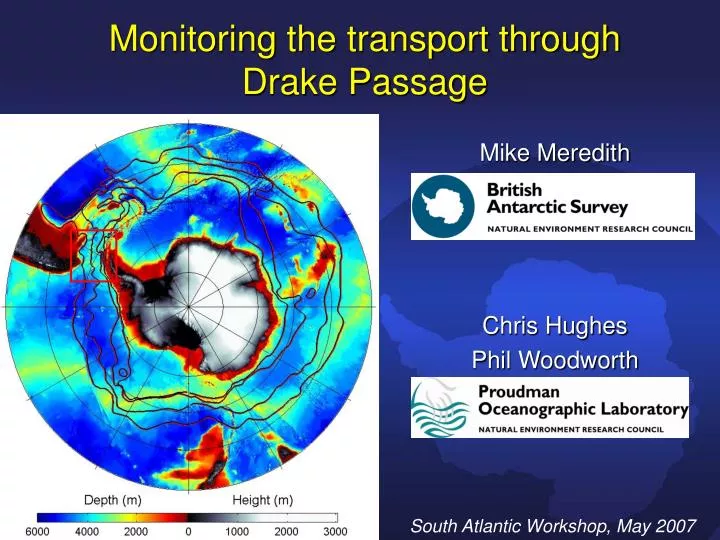
Monitoring the transport through Drake Passage. Mike Meredith Chris Hughes Phil Woodworth. South Atlantic Workshop, May 2007. Overview:-. Why? Drake Passage transport variability on a range of timescales:- 1) subseasonal 2) seasonal 3) interannual 4) secular (briefly)

E N D
Monitoring the transport through Drake Passage Mike Meredith Chris Hughes Phil Woodworth South Atlantic Workshop, May 2007
Overview:- • Why? • Drake Passage transport variability on a range of timescales:- • 1) subseasonal • 2) seasonal • 3) interannual • 4) secular (briefly) • What is forcing and limiting the observed transport variability • The present and possible future state of monitoring - minimum requirements for a Drake Passage monitoring system?
Why? :- • Drake Passage is a key chokepoint for the world’s largest current, the Antarctic Circumpolar Current (ACC). • Heat, salt, mass, freshwater, nutrients etc. are moved between the Atlantic, Pacific and Indian Oceans, with consequences for global climate, ecosystems etc. => Therefore important to know what variability the oceanic circumpolar transport exhibits on a range of timescales, and how it interacts with lower latitudes.
Why? Large quantities of mass, heat, salt etc moved around Southern Ocean, with links to lower latitudes. Divergence between chokepoints requires knowledge of the chokepoint transports. How do these change? (Ganachaud, Wunsch)
How do we monitor the transport?Lots of methods have been tried… • Repeat hydrographic sections (CTD, ADCP, LADCP) • Repeat expendable bathythermograph (XBT) sections • Current meter arrays • Tide gauge data • Bottom pressure recorders (BPRs) • Inverted echo sounders (IESs) • Satellite altimetry • Satellite gravity • etc
ND2 How do we monitor the transport variability? • Lots of different ways… • But one of the most useful (for reasons that will become clear) is to use bottom pressure recorders (BPRs) and tide gauges • Antarctic network is not massive, but good coverage around >½ continent • ND2 and SD2 first deployed during WOCE; now nearly 20 years of data.
How do we monitor transport variability? • Models suggest that sea level/bottom pressure adjacent to Antarctica should be a good index of circumpolar transport • Also that transport changes are genuinely circumpolar on these timescales, and strongly steered by bathymetry (Hughes, Meredith & Heywood, JPO, 1999)
BPRs deployed from ship; depths typically 1000-3000m Deployments typically of 1-2 years duration – main use is for subseasonal and seasonal variability.
Subseasonal timescales OCCAM ¼º (Hughes et al., GRL, 2003; see also Aoki, GRL, 2002) • Highly coherent. • No discernable lag between forcing and response. • No discernable lag around Antarctica. • Strongly related to (predicted) Drake Passage transport.
Forcing for circumpolar transport variability is the Southern Annular Mode • See-saw in barometric pressure between Antarctica and lower-latitudes. • Dominant mode of extra-tropical atmospheric variability in Southern Hemisphere. • Dominant timescales are ~10 days and longer. • Increasing, due to likely anthropogenic causes (e.g. Thompson and Solomon, Science; 2002; Marshall et al. GRL, 2004). 850-hPa height regressed on SAM index
What is forcing the variability? • Correlation of south Drake Passage BPR data with eastward wind from NCEP reanalysis • Shows genuine circumpolarity of forcing
Subseasonal timescales So what is the forcing for the northern Drake BPRs …? Equatorial/tropical Pacific winds, rather than circumpolar SAM.
Subseasonal timescales Related to waves propagating along shelf and slope of South America. Evidence of baroclinicity in wave structure => choice of deployment depth is critical (unlike south Drake) (Hughes and Meredith, 2006)
North Drake BPR data also shows strong correlation with transport of Malvinas Current at ~40˚S. Lag is approximately 2 weeks – a different mode? (Vivier, Provost and Meredith, JPO, 2001).
Seasonal timescales (Meredith et al., GRL, 2004) • Circumpolar winds have strengthened in recent decades, with change strongly seasonally modulated. • Trends in month-by-month BPR data agree with those of the SAM. • => changes in the seasonality of the circumpolar winds are inducing changes in the oceanic circumpolar transport. (Anthropogenic?)
Interannual timescales (Meredith et al., 2004) • Faraday tide gauge is best dataset for interannual variability • Annual means show significant correlation with SAM, and also OCCAM transport, despite baroclinic variability • Range of transport is quite small (~7 Sv, c.f. ~20 Sv from CTDs) • Aliassing is clearly an issue with CTD sections
So what sampling interval do we need to get reliable annual means? (Meredith and Hughes, GRL, 2005) • Answer is: < 7 days, for 95% level! • And this presumes zero measurement error… • In practice, need continuous data from in situ instrumentation (BPRs etc)
Interannual timescales • Sampling requirement alone demands measurement interval of shorter than 1 week. • Significant measurement errors mean that even more rapid sampling is required. • Which means that repeat CTD/XBT/ADCP sections will not capture true seasonal or interannual variability. • Neither will altimetry along a single groundtrack. • In practice, need continuous data from in situ sources. • Some combination of BPRs/tide gauges/moorings etc is required
Why does the ACC vary so little on interannual timescales? • ACC accelerates as eastward wind stress increases • Circumpolar Eddy Kinetic Energy then begins increasing, limiting the increasing transport of the ACC. (Meredith & Hogg, GRL, 2006)
Secular changes (Fyfe & Saenko, 2005) • Winds over Southern Ocean have increased dramatically in recent decades… • Has ACC accelerated in response? • And/or moved southward? • Coarse-resolution models suggest there should be a change…
But how would we know…? • On interannual timescales, a change in SAM index of 1 gives a change in ACC transport of around 6 Sv… • If same relationship holds true for longer timescales (?), acceleration in ACC due to trend in SAM would be small compared to aliassing and measurement error. • And tide gauges have trends all their own.
The Present: monitoring is rather disparate, both spatially and scientifically France CM UK CTD + BPR (WOCE SR1b) US PIES WOCE SR1 Russia CTD Spain CTD Argentina CTD US XBT/ADCP WOCE A21
The Future: • More strategic thought about what the separate elements are telling us, and how they are connected. • Commit to having instrumentation in situ long-term. • Special attention to northern boundary of Drake Passage, and signals passing to western boundary of South Atlantic. • Trends (how?). • Smarter use of remote sensing (inc. GRACE?). • Monitor temperature and salinity concurrently with velocity if want variability in heat & freshwater fluxes.