Download
1 / 59
600 likes | 636 Views
Ground-based Measurements. Measurements Retrieving the Desired Information Comparison Between Instruments Satellite Validation Toward Model-Measurement Comparison. Prepared by: Dr. Stella M L Melo University of Toronto.

E N D
Ground-based Measurements Measurements Retrieving the Desired Information Comparison Between Instruments Satellite Validation Toward Model-Measurement Comparison Prepared by: Dr. Stella M L Melo University of Toronto Part of the material presented here was provided by Prof. K. Strong
Points: • Understanding what is measured • Extracting the desired information from the measurement • Comparing measurements made using different techniques • Measurements and models…
Measurement: • Remote sensing/sounding: • a means of obtaining information about an object or medium “without coming into physical contact with it”. • This generally involves the measurement of EM radiation that has interacted with the object or medium of interest.
Interaction of Radiation with Gases: • Ionization – dissociation (UV) • Electronic transition (UV- visible) • Vibrational transitions (infrared) • Rotational transitions
Measurement: • Remote sensing/sounding techniques can be classified by the type of measurement and the spectral region. • ACTIVE vs. PASSIVE • IMAGING vs. NON-IMAGING vs. • WAVELENGTH OF RADIATION MEASURED
REMOTE SENSING AND SOUNDING TECHNIQUES PASSIVE IMAGING NON-IMAGING SOUNDING IMAGING NON-IMAGING SOUNDING EXTINCTION RANGE POWER BACKSCATTER REFLECTED THERMAL EMISSION SUNLIGHT RADIATION SCATTERING IMAGING LASER RADAR SCATTER- AERIAL VIS/ THERMAL PASSIVE RADAR PROFILER ALTIMETER OMETER PHOTO- NEAR-IR INRARED MICROWAVE (m-WAVE) (VIS/IR) (m-WAVE) (m-WAVE) GRAPHY SCANNER SCANNER RADIOMETER LIDAR SIDE- SYNTHETIC (VIS/IR) LOOKING APERTURE AIRBORNE RADAR RADAR (SAR) LASER (SLAR) RADIOMETER SPECTROMETER BROAD- SELECTIVE HETERO- HETERO- BAND FILTER DYNE DYNE (VIS/IR) (VIS/IR) (m-WAVE) (VIS/IR) ACTIVE RADAR (m-WAVE) FABRY- FOURIER GRATING PEROT TRANSFORM (UV/VIS/IR) (VIS/IR) (VIS/IR)
Measurement: • Passive Systems • These generally measure the extinction, emission, or scattering of radiation in order to retrieve atmospheric properties. • Radiometers – isolate bands of natural radiation using some form of spectral filter; • Spectrometers – disperse natural radiation into its constituent wavelengths over a finite spectral range or use interference effects to obtain spectral information; • Monochromatic LASER Techniques - LASER is used in a passive mode in a heterodyne system, serving as a local oscillator;
Measurement: • Active Techniques (1)- radio (microwave) spectrum RADAR (RAdio Detection And Ranging) (2)-visible and infrared spectrum • LASER (Light Amplification by Stimulated Emission of Radiation) • LIDAR (LIght Detection And Ranging)
Gas Absorption/Emission Spectroscopy • Absorption and emission spectra provide a means of identifying and measuring the composition and temperature of the atmosphere. http://ess.geology.ufl.edu/ess/notes/050-Energy_Budget/absorbspec.jpeg
ds I + d I l l I l Gas Absorption/Emission Spectroscopy Four processes will change the intensity of the EM radiation as it passes through the volume: A – absorption from the beam (depletion term) B – emission by the material (source term) C – scattering out of the beam (depletion term) D – scattering into the beam (source term)
What is measured Passive remote sounding instruments are used to observe extinction, emission, and scattering of natural radiation. Scattering Extinction Emission
Measurements Techniques • DOAS • Retrieving vertical distribution of constituents from ground-based measurements • Temperature form Airglow and from Lidar
Ground based Measurements: DOAS • Differential Optical Absorption Spectroscopy – DOAS • a method to determine concentrations of trace gases by measuring their specific narrow band absorption structures in the UV and visible spectral region [Platt and Perner, 1983; Platt, 1994].
DOAS • Differential absorption cross-sections of some trace gases absorbing in the UV/vis wavelength region. • On the right axis the detection limits of the trace gases is listed together with the typical light path lengths used to measure them.
DOAS Varies slowly with l
DOAS: NO3 • Example of NO3 analysis: • Daytime reference and night time spectra to be analyzed • The division of the two spectra with a low-pass filter • The fit of NO3 to the OD spectrum, d) Residual • e) and f) NO3 and H2O cross-section From: Allan et al., JGR 105, 2000
Viewing Geometry • Direct sun • Zenith sky • Bright-sky (less commonly used?) Zenith Sky Direct Sun
Viewing Geometry • Direct Sun • Longer path through the troposphere (than zenith) • Air mass factor calculation normally requires only geometric considerations • Clear sky conditions are required… • Zenith Sky • Longer path through the stratosphere • Possible to measure absorption at SZA greater than 90 • Any weather conditions • Air mass calculation involves complex scattering geometry… • Bright-Sky • Instrument points towards the brightest part of the sky • Increased sensitivity to aerosol scattering…
Zenith sky configuration: • Particularly sensitive to stratospheric absorbers • For the analysis of DOAS measurements using direct or scattered solar radiation traversing the atmosphere, the so-called air mass factor concept has been developed (see e.g. Noxon et al. [1979], Solomon et al. [1987b]). • Since the measured slant column density (SCD), the integrated trace gas concentration along the light path, strongly depends on the solar zenith angle (SZA), it is advantageous to convert the SCD into a vertical column density (VCD), the vertically integrated trace gas concentration. • This conversion is usually performed by dividing the SCD by the air-mass factor (AMF): VCD = SCD(SZA) / AMF(SZA) (apparent SCD)
NO3 Column density (/1014 molecule.cm-2) SZA DOAS: NO3 Figure 3. Examples of the variation in the vertical column density of NO3 obtained from zenith sky measurements during field campaigns carried out at Weybourne, Mace Head, Tenerife, Cape Grim and Norway. From: Allan et al., JGR 107, 2002
DOAS: NO3 Figure 6. Examples of profile retrieval from NO3 vertical column density measurements made on 3 February 1999 (triangles) and 15 February 1999 (circles) at Cape Grim, Tasmania. From: Allan et al., JGR 107, 2002
O3 DOAS fit By Elham Farahani
Ozone – Eureka 1999 Fig. 1. Ozone vertical column densities measured with the University of Toronto UV-visible spectrometer, compared with data from sondes, a Brewer spectrophotometer operated by the Meteorological Service of Canada, and the TOMS satellite instrument. Melo et al., ASR, 2004
NO2 DOAS fit By Elham Farahani
NO2 Vertical column Fig. 2. NO2 vertical column densities at SZA=90° observed with the UV-visible spectrometer. Values were obtained assuming a reference column density of 1.46x10¹⁶ molec.cm-2. Melo et al., ASR, 2004
NO2 Vertical distribution NO2 slant column (x1017 molec cm-2) (K. E. Preston et al., J. Geophys. Res. 102, 19089, 1997)
Retrieval or inversion theory • The direct or forward problem: • - A detector measures a signal S = f(T) which is generated by the interaction of radiation with the target (atmosphere, clouds, etc.). • given properties of the target, calculate signal • The inverse problem: • Want to determine properties of the target, given by the inverse function T = f-1(S). • given signal, calculate properties of the target
Solving the inverse problem: • Solving the inverse problem is complicated by a number of difficulties: • (1) Non-uniqueness of the solution: • several unknown parameters, which can be combined in different ways to generate the same observed signal. i.e., have several solutions T1 = f-1(S), T2 = f-1(S), etc. • (2) Discreteness of the measurements when the measured quantity is a smoothly varying function. e.g., T is a function of height z, while S is measured at discrete levels over some range of heights, so where K(z) is called a kernel function or a weighting function. • (3) Instability of the solution due to errors in the observations S. e.g., If is the error on S, then where can produce a large change in the retrieval of T(z).
NO2 Vertical distribution The inversion problem consist of expressing the unknown profile x in terms of the observations y: y – measurements - SCD F – forward model b – model parameter ey – measurements error y=F(x,b)+ey Direct inversion? Well, the problem is under-constrained… There is no unique solution – choose the “optimal” solution
NO2 Vertical distribution - For the purpose of retrieval, the inverse problem can be reformulated in a discrete form (Rodgers, 1976): y=KxwhereK=dy/dx The rows of the K matrix are know as weighting functions and each one corresponds to a different measurement. • Rodgers (1976) reviews a number of different methods • Sequential estimation was chosen for this study: • Solving the optimal estimation equation sequentially.
NO2 Vertical distribution • Vertical profile can be retrieved using optimal estimation sequentially [Rogers, 1990] • minimizes the difference between measured and calculated slant column values as a function of SZA to determine the optimum solution profile for each set of twilight spectra. • is based on sequentially combining a set of independent measurements by taking a weighted average, using the measurement errors as weights. • does not require iterations • includes a formal treatment of errors. • Vertical resolution: 5 to 7 km from 10 to 35 km altitude.
Retrieval • Optimal estimation: • Combining two independent measurements, x1 and x2, by taking the average, using the inverse of the error covariances, S1 and S2, as weight Covariance matrix of x - Those equations can then be used to invert slant column measurements
Retrieval x=K-1y The measurement error inverse covariance S-1e can be mapped into profile space using the K matrix: KTS-1eK. x0 – a priori with error covariance Sx : ^ ^ Covariance of x Simplifying: Can be solved sequentially
Retrieval • The measurements are treated as m scalars, yi, with corresponding standard deviation si. • The a priori, x0, is the first guess of the vertical profile • It is sequentially updated or improved using one weight function Ki and one measurement yi at a time • The error covariance S is retrieved simultaneously with the vertical profile
Does it works? • CMAM vertical profiles of NO2 concentration for Vanscoy for a set of SZA range during both twilights are used to generate SCD as a function of SZA (Chris McLinden). • Those SCD are used into a retrieval code to retrieve back the NO2 vertical distribution at sunrise and sunset (SZA=90°); • Both the forward model and the box model employed in the retrieval are independent from either CMAM or Chris McLinden models. • The “a priori” used in the retrieval is also independent of CMAM.
Information content: • Smoothing CMAM using Rodgers aproach (Rodgers and Connar, JGR 108, Vol D3, 4116, 2003): assume CMAM is the “true” (Xh), the smoothed profile (Xs) will be given by: Xs=Xa + A(Xh – Xa); • Xa represents the “a priori” adopted in the retrieval and A represents the Averaging Kernels.
Adding Tropospheric NO2 Zenith viewing geometry: low sensitivity to troposphere:
Using measurements: Fig. 4. NO2 a priori, measured, and retrieved absolute slant column densities for March 31, 1999 (day 90) measured at Eureka. Values were obtained assuming RCD=1.46x10¹⁶ molec.cm-2. Melo et al., ASR, 2004
Using real measurements Eureka 1999 Fig. 5. Left plot: retrieved NO2 profiles for SZA=90° on March 31st, 1999 (day 90) compared with the initial profile. Right plot: error in the a priori and retrieved profiles. Values were obtained assuming RCD= 1.46x10¹⁶ molec.cm-2. Melo et al., ASR, 2004
NO2 and O3 – Eureka 1999 Fig. 7. O3 partial pressure measured using a sonde launched from Eureka at 23:27 UT on March 31, 1999 (day 90). NO2 Vertical distribution
NO2 from different platforms Figure 1. The NO2 slant columns measured with the ground-based UV-visible spectrometer on August 24, 1998 (MANTRA) and the fitted values. The symbols represent measured values while the lines represent retrieved values. Lower plot: the percent difference ((measured-fitted)/measured), sunrise (diamonds) and sunset (squares). Melo et al., A-O, Submitted
MANTRA Balloon Campaign • MANTRA is conducted at Vanscoy, Saskatchewan (52°N, 107°W): - August 24, 1998, - August 29, 2000, - September 3, 2002, - NEXT: August 2004 • Instruments of interest here: balloon-based SPS, SAOZ, and DU-FTS, the ground-based UT Spectrometer; and the sondes. • In this work we report on vertical profiles of T, O3, NO2, N2O, CH4, and HCl concentrations .
MANTRA Scientific Objectives • To measure vertical profiles of the key stratospheric gases that control the mid-latitude ozone budget. • To combine these measurements with historical data to quantify changes in the chemical balance of the stratosphere, with a focus on nitrogen compounds. • To compare multiple measurements of the same trace gases made by different instruments. • To use the measurements for validation and ground-truthing of Odin, ENVISAT, and SCISAT-1. http://www.atmosp.physics.utoronto.ca/MANTRA
NO2 - Comparing with models • What kind of models? • CTM - MEZON (Model for Evaluating oZONe Trends) global chemistry-transport model. • horizontal resolution of 4° in latitude and 5° in longitude • Vertical: the model spans the atmosphere from the ground to 1 hPa • driven by wind and temperature fields provided by the UKMO • initial conditions for the trace-gas concentrations have been taken from the UARS • lightning source of NOx is prescribed • Rozanov et al. (1999) and Egorova et al. (2001, 2003) • GCM – CMAM Canadian Middle Atmosphere Model (CMAM) • upward extension of the Canadian Centre for Climate Modeling and Analysis (CCCma) spectral General Circulation Model (GCM) up to 0.0006hPa (roughly 100 km altitude).