Download
1 / 21
210 likes | 305 Views
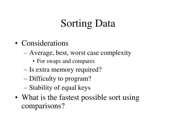
Sorting Data. Considerations Average, best, worst case complexity For swaps and compares Is extra memory required? Difficulty to program? Stability of equal keys What is the fastest possible sort using comparisons?. Elementary Sorting Methods Complexity O(n 2 ), All are Stable.

E N D
Sorting Data • Considerations • Average, best, worst case complexity • For swaps and compares • Is extra memory required? • Difficulty to program? • Stability of equal keys • What is the fastest possible sort using comparisons?
Elementary Sorting MethodsComplexity O(n2), All are Stable • Bubble Sort (N(N-1)/2)comparisons, about N(N-1)/4 swaps) • Selection Sort (N(N-1)/2 comparisons, N-1 swaps) • Minimizes the number of swaps • Worst case equals average case • Insertion Sort (N(N-1)/4 comparisons and copies) • Good for lists that are nearly sorted (O(N) best case)
Bubble Sort Pairwise compares of adjacent elements; swap where necessary pass = 0; swaps = true; while (pass < n && swaps == true) { swaps = false; for (index=0; index<n-pass; index++) { if (sortArray[index] > sortArray[index+1]) { swap(sortArray, index, index+1); swaps = true; } } pass++; }
Selection Sort Find Minimum n-1 times for (i=0; i<n-1; i++) { minimum = i; for (j=i+1; j<n; j++) { if ( sortArray[j] < sortArray[minimum]) minimum = j; } swap(sortArray, i, minimum); }
Insertion Sort Insert next entry into a growing sorted table for (i=1; i<n; i++) { j = i; save = sortArray[i]; while (j>0 && save < sortArray[j-1]) { sortArray[j] = sortArray[j-- - 1); } sortArray[j] = save; }
Proof by Induction • Select Base Case (n = 1) • State the Hypothesis (assume for n=k) • State what is to be proved (prove for n=k+1) • Example: Base case: For n = 1, 1 = 1 * 2 / 2 = 1 Hypothesis: Assume for n=k, 1 + 2 + … + k = k * (k+1)/2 To Prove: 1 + 2 + … + k+1 = (k+1) * (k+2) /2 1 + 2 + … + k+1 = 1 + 2 + … + k + (k+1) By the hypothesis, this equals k * (k+1)/2 + (k+1) = (k+1)(k/2 + 1) = (k+1)(k/2 + 2/2) = (k+1)(k+2)/2 Therefore by induction, the relationship holds for all positive k >= 1
RecursionUseful for advanced sorts and for divide & conquer algorithms • Relationship to mathematical induction • Key design principals • Relationship between algorithm(n) and algorithm(m) where m<n. • Base Case (How does it stop?) • When is it useful? What is the overhead? • Relationship between n and m • Tail recursion with a single recursive call • Replace by manually creating stacks • Examples • simple loop, factorial, gcd, binary search, tower of hanoii
Recursion Examples • Factorial: 5! = 5 * 4! • Greatest Common Denominator: gcd(x,y) = gcd(y%x,x) if x<y • Binary Searchint binSearch( array, low, high, value) { if (high – low <= 1) return -1; // Base case middle = (low + high) / 2; if value < array[middle]) binSearch(array, low, middle-1, value) else if value > array[middle]) binSearch(array, middle+1, high, value) else return middle; }
Breaking the O(N2) BarrierBased on either bubble or insertion sortComplexity from O(N7/6) to O(N3/2) based on gap selection • Shell Sort while (gap > 0) { for (index=gap; index<n; index++) { temp = sortArray[index]; compareIndex = index; while(compareIndex>=gap && sortArray[compareIndex-gap]>=temp) { sortArray[compareIndex]=sortArray[compareIndex-gap]; compareIndex -= gap; } sortArray[compareIndex] = temp; } adjustGap( gap ); // different patterns (/=2, (gap-1)/3, (gap+1)/2 }
Shell sort (based on bubble) int index; while (gap > 0) { swaps = true; while (swaps) { swaps = false; for (index = 0; index < gap; index++) { if (sort[index] > sort[index + gap]) { swap(sort, index, index + gap); swaps = true; } } } adjustGap( gap ); }
Merge SortAlways O(N lgN) but need more memory • Merge Sort void mergeSort(double[] sortArray, int low, int high) { int mid = (low+high)/2; if (low == high) return; mergeSort(sortArray, low, mid); mergeSort(sortArray, mid+1, high); merge(sortArray, low, mid, high); } • Merge method must: • Allocate an array for copying • Merge two sorted arrays together • Copy back to original array
Merge method void merge(double[] sort, int low, int middle, int high) { int n = high – low + 1, int lowPtr = low, highPtr = middle+1, spot = 0; double work = new double[high – low + 1]; while(low <= middle && high <=top) { if (sort[lowPtr]<sort[highPtr]) work[spot++] = sort[lowPtr++]; else work[spot++] = sort[highPtr++]; } while (lowPtr<=middle) work[spot++] = sort[lowPtr++]; while (highPtr <= top) work[spot++] = sort[highPtr++]; lowPtr = low; for (spot=0; spot<high-low+1; spot++) sortArray[lowPtr++] = workArray[spot]; }
Analysis of Merge Sort 16 8 8 4 4 4 4 2 2 2 2 2 2 2 2 Work at each level totals to 16, lg 16 = 4 levels, complexity = 16 lg16
Quick SortO(NlgN) average case, in place void quickSort(double[] sortArray, int left, int right) { if (right <= left) return; double pivot = sortArray[right]; int middle = partition(sortArray, left, right, pivot); quickSort(sortArray, left, middle-1); quickSort(sortArray, middle+1, right); } • Refinements to avoid O(N2) worst case and speed up. • Choice of pivit • Combining with insertion sort • Other uses (find the kth biggest number).
Quick Sort Partitioning int partition(double[] sortArray, int left, int right, int pivot) { int origRight = right; left -= 1; for (;;) { while(sortArray[++left] < pivot); while(sortArray[--right] > pivot); if (left >= right) break; swap(sortArray, left, right); } swap(sortArray, left, origRight); return left; }
Radix Sort (First Version) • Choose the number of buckets (b) • Drop next significant part of data into buckets • Gather data from buckets back into original array • Repeat the above two steps, finishing at the most significant piece of data • Notes • Maximum memory needed for each bucket • Complexity: O(p * 2n) where • p = (Max + b – 1)/b • 2n because dropping and gathering touches each element twice
Radix Sort example Notes: Each pass is a digit of the data (x / 10 (pass – 1)) % 10 Two passes because largest number < number of buckets squared Complexity is: O( 2pn) = O(pn) where p is the number of passes In this case, only two elements are in each bucket, but we couldn’t depend on that in the general case
Refined Radix Sort • Create and initialize an array (Counts) of size buckets + 1 • Initialize the array to zeroes • Store actual bucket sizes into Counts array (starting index = 1) • Perform a prefix sum on Counts array to compute starting offsets • Use Counts array to drop elements into a second array of numbers • Advantages: • Use alternating arrays to avoid the gather operations • Only two times the memory is needed • Complexity: O(p(2n + 2b)) = O(p(n+b)) • Notes: • Increased buckets can reduce the number of passes, but prefix sum overhead will limit performance benefits. • Radix sort does no comparisons , so O(n lg n) limitation doesn’t apply.
Refined Radix Example • Dump from original array to alternate array • No gather operation needed • Index to store into count array is one bigger than the bucket. count array index 5 in the above example has a count of 1 because it corresponds to bucket 4.
Optimal Comparison Sort • There are n! possible comparison sorts • All sorts can be modeled with a decision tree • Optimal sort will be completely balanced • Depth of the balanced decision tree is O(lg(n!) Decision Tree compare compare compare <= > <= > > <=
Prove optimal sort <= O(n lg n) • Optimal comparison sort <= O(n lg n) lg (n!) = lg(n) + lg (n-1) + lg (n -2) + … + lg(1) < lg n + lg n + lg n + … + lg n = n lg n = O(n lg n) • Optimal comparison sort >= O(n lg n) lg (n!) = lg(n) + … + lg(n/2+1) + lg(n/2) + … + lg(n/4+1) + lg(n/4) + … + lg(n/8+1) + … > n/2 lg(n/2) + n/4 lg(n/4) + n/8 lg(n/8) + … = n/2 lg(n) – n/2lg 2 + n/4 lg(n) – n/4lg 4 + n/8 lg n – n/8 lg 8 ≈ n lg (n) – ½ n – 2/4 n – 3/8 n – 4/16 n - … = n lg (n) – n (1/2 + 2/4 + 3/8 + 4/16 + … = n lg n – 2n But O(n lg n – 2n) = O(n lg n) • Therefore optimal sort = O(n lg n) • The series is well known: ½ + 2/4 + 3/8 + … = ∑ n/2n ≈ 2 • Proof: S(2n) – S(n) = S(n) = 1 + 1 + 6/8 + 8/16 + 10/32 – ½ - 2/4 – 3/8 -…= 1 + ½ + ¼ + 1/8 +…= 2