Download
1 / 20
210 likes | 351 Views
Spatial Statistics in Ecology: Area Data. Lecture Four. Recall and Introduction to Area Data. Recall that we have visualized, explored and modeled point patterns and continuous processes Many of the same concepts that you have previously learned apply to area data

E N D
Spatial Statistics in Ecology: Area Data Lecture Four
Recall and Introduction to Area Data • Recall that we have visualized, explored and modeled point patterns and continuous processes • Many of the same concepts that you have previously learned apply to area data • Think of area data like a continuous process that is separated in zones
Can you think of some types of area data that ecologists might use?
Types of Area Data • Recall that area data is either grid – raster format or irregular – vector format • Area data must be continuous like states in a country – this is called “contiguity” • Areas must be contiguous to create the spatial weight matrix that is used to study first order effects • Areas that are not contiguous can still be studied for second order effects
Patterns in zonation • Each area is assumed to have a fixed value or mean value • We are not interested with areal data in predating the value of an attribute in areas which it has not been sampled • Instead we are interested in how the zones vary and the type of pattern that arises across zones Proportional symbols map
Visualizing area data Area data is mapped using the choropleth map or using proportional symbols Grid or lattice data Irregular zone data
Exploring Area data: Proximity • The first issue to deal with when using area data is PROXIMITY • Proximity refers to how to measure how close a unit is to another unit when they are irregularly shaped and do not have obvious grid like centroids
Proximity Length of boundary Some examples are: • Centroids • Common boundaries • Length of boundaries • Hybrid measures such as shared boundary + distance between centroids centroids Common boundary
Spatial Weight Matrices • Proximity is used to create a spatial weight matrix • (n x n) proximity matrix W, each of whose elements wij, represents a measure of the spatial proximity of areas Ai and Aj
Kernel Estimation • For area data Kernel estimation requires a fixed centroid as it cannot be used to look at irregular areas. • Thus, kernel estimation is more appropriate for grids and lattice data or data with obvious centroids • In this case Kernel estimation is almost the same as it was for spatially continuous data
Second-order: AUTOCORRELATION • Remember the variogram? The correlogram in typically used to explore spatial dependence of area data • When applied to area data it is formally called spatial autocorrelation • Autocorrelation involves correlation between values of the SAME variable at different spatial locations
Conceptual Geary’s c Moran’s I Similar, regionalized, smooth, clustered 0 < C < 1 I > 0* Independent, uncorrelated, random C = O I < 0* Dissimilar, contrasting, checkerboard-like C > 1 I < 0* Note 0* = 1/n(n-1) where n is the number of objects Autocorrelation Moran’s I represents the overall agglomerative patterns of areas (are areas of like value clumped together or dispersed Geary’s c explains similarity or dissimilarity (is it possible to predict from one area what the value will be at a neighboring area).
Both Moran’s I and Geary’s C an be used to create correlograms showing the lag to lag (distance) spatial dependence between areas The correlogram
Example correlograms What can you tell about the spatial dependence of these 3 variables?
Non-spatial regression models Suitable if there is no spatial dependence First produce a correlogram If there is no dependence proceed with regression Spatial regression models If there is spatial dependence than use a spatial regression model SAR or CAR models Modelling area data
Example: Ireland Blood Type A • How is blood type A distributed in Ireland? Samples were taken from 55000 people in 26 counties • How does the proportion of people with blood type A vary across counties?
Summary: Lecture Four • Area data differs from continuous processes in that we look at variation in the mean value of an area to discover patterns between zones • First-order effects are studied by kernel estimation or spatial autoregressive models • Second-order effects are considered using Moran's I and Geary’s and by producing correlograms