Download
1 / 23
230 likes | 372 Views
Network Formation in the Presence of Contagious Risk. Éva Tardos Cornell University Joint work with Larry Blume, David Easley, Jon Kleinberg and Bobby Kleinberg. Models of Network Formation. Why do complex networks look the way they do? Two classes of models: Probabilistic Strategic.

E N D
Network Formation in the Presence of Contagious Risk Éva Tardos Cornell University Joint work with Larry Blume, David Easley, Jon Kleinberg and Bobby Kleinberg
Models of Network Formation Why do complex networks look the way they do? Two classes of models: • Probabilistic • Strategic Corporate e-mail communication (Adamic and Adar, 2005) Book recommendations (Leskovec-Adamic-Huberman 2006)
Models of Network Formation Probabilistic: Links form by simple probabilistic rules. • Preferential attachment: Link to other nodes with prob. proportional to their degrees [Barabasi-Albert 1999]. • Small-world models: Link to other nodes with probability decaying in distance [Watts-Strogatz 1998, Kleinberg 2000]. Corporate e-mail communication (Adamic and Adar, 2005) Book recommendations (Leskovec-Adamic-Huberman 2006)
Models of Network Formation Strategic (e.g. [Jackson-Wolinsky 1996, Bala-Goyal 2000]): • Nodes can construct a subset of the possible links incident to them. • They receive payoffs based on the structure of the overall network that forms. Corporate e-mail communication (Adamic and Adar, 2005) Book recommendations (Leskovec-Adamic-Huberman 2006)
Strategic Network Formation Parameters > 0 and 0 < < 1. Node i'spayoff is i= - di +ji dist(I,j) where di is degree • A network is stable if no node can change its behavior to increase its payoff, given the choices of other nodes, e.g., • Node i can't strictly increase its payoff by deleting all its links. • If (i, j) isn't an edge, then adding (i, j) can't raise the payoffs of both i and j (at least one strictly). ? ? ? 0, -++2 , -2+2
Our game: different payoff • Standard payoff: • cost for link di • benefit from reaching others ji dist(I,j) • Our model: • benefit from link • Danger from being connected to others
Financial Networks Financial networks [Allen-Gale 2000, Haldane-May 2011] • Nodes benefit from transactions with others, but ... • Counterparty risk: If X defaults on Y, this can hurt Y (and spread contagiously to other counterparties of Y ). Network of overnight loans among banks (Bech and Atalay, 2008)
Disease Epidemics Human contact networks • In the presence of an epidemic disease, people will alter their contact patterns to restrict more to in-group members. • Evidence in case of HIV/AIDS for sexual contacts and needle-sharing [Jacquez et al 1988, Barnard 1993]. Network of sexual contacts (Potterat et al, 2002)
Covert Organizations Social networks in covert organizations. • Links are useful for coordinations, but ... • If one member is compromised, discovery of others can spread across links [Gutfraind 2010]. Terrorist network (Krebs 2001)
Our Model Link formation: • Players V can form up to bilateral relationships with others, obtaining a benefit of a > 0 from each. • Resulting in undirected graph G = (V; E). A failure process then spreads through the graph: • Each node fails spontaneously with probability q > 0. • Failure spreads along each edge with probability q > 0. • Failed nodes lose link benefits and also incur cost of b < 0.
Payoffs Let Adenoting the probability node A fails, A 's payoff is A = a dA (1 -A ) - b A : We compare graphs G according to min-welfare: min A A • Socially optimal G: maximizes min-welfare over all graphs. • Also look at best/worst min-welfare of stable graphs. Stable = No node wants to delete all incident edges; no non-edge pair wants to link. A
Assumptions ? a > bqp. a < bp. a < bq. ? ? • Assume that all of these bounds hold by a wide margin. • Condition P(): • -1 bqp < a < min(bp; bq):
Main Results The optimal min-welfare is (1 + f ())a/p for a non-negative fn f () 0. • Socially optimal graphs are positioned just past a natural phase transition in the behavior of the payoffs. • Exposes a difference between clustered and anonymous market structures. For a sufficiently large number of nodes, the largest min-welfare of a stable graph is g() a/p for a fn g() 0. • Stable graphs involve slightly too much linking, which quickly burns away almost all the available payoffs. • A type of tragedy of the commons, with survival probability serving as the shared resource that gets overconsumed.
Techniques: life-edge subgraph Nodes fail independently with probability q > 0. Edges fail independently with probability p > 0. • Picture the choice of failed edges being made first, before nodes fail. • Results in a live-edge subgraph. • A node fails, if any node in his life-edge component fails
Special case: click • G is a complete graph. • Live-edge subgraph is a sample from the random graph Gn,p. Theorem: If p =(1-x)/n for fixed x, the probability a node A 's component exceeds size c is exp(-c). Theorem: If p =(1+x)/n for fixed x, with high probability a component of size (x)n. Expected max comp n/2 0 .7 1 1.4 Expected degree
Life-edge components in general Let G be a graph with minimum degree d, and declare each edge to be life with probability p, where pd = 1 + x for some fixed x > 0. • Then for any node A , there is a constant prob. that A's live-edge component contains >d nodes, for a constant . A consequence (for fixed x > 0, with p; q; small): • For all nodes to get payoff (1 + x)a/p, need degree (1 + x)/p • This means each node A has a constant probability of being in a large live-edge component high a probability of failure and hence a negative payoff. Corollary: fn f () 0 such that no network can have min welfare >(1 + f ())a/p (critical payoff: a/p)
Proof idea A To show (high prob.) existence of a giant component [Karp 1990]: Imagine performing breadth-first search to discover A's component. • At the start, we remove one node from the BFS queue and add 1 + x nodes in expectation. • So initially, the length of the BFS queue behaves like a random walk with positive drift
Super critical payoff possible? Question: Is it possible to reach payoff (1+f ())a/p, where f () can go to 0 with ? (assume p=q) yes • clustered market? union of disjoint cliques of size (1 + f())/p each. • Anonymous market? random d-regular graph on n nodes, with d = (1 + f())/p. no
Proof idea: clustered vsanymous Start with degree 1/p, and ask: is it a good idea to increase the degree to (1 + x)/p for some very small x? Compare the payoff increase from links with payoff decrease from failure. • A 's gain in payoff from the links is ax=p. • A 's loss in payoff is b times the increased probability of failure. • First-order approximation of payoff loss via differentiation.
Stable graphs Why is the optimal union of cliques not stable? • Two nodes A and B in different cliques will want to connect. • A and B pass on increased risk to other nodes in their cliques, • reducing payoffs of these other nodes: a negative externality. Theorem: the union of slightly larger cliques is stable (with near-zero node payoffs). Theorem: min-welfare of a stable graph of max degree is g() a/p for a function g() 0.
Proof idea: stable graphs Theorem: min-welfare of a stable graph of max degree is g() a/p for a fn g() 0. failure probabilities A and B • B doesn’t want edge (A,B): • benefit a < loss bpAhence a/bp < A Payoff for such high risk nodes A = a dA (1 -A ) - b A < a dA - a/p hence needs degree (1+g()) A B
Proof idea: stable graphs Theorem: min-welfare of a stable graph of max degree is g() a/p for a fn g() 0. Payoff for such high risk nodes A = a dA (1 -A ) - b A < a dA - a/p hence needs degree (1+g())/p Low risk nodes • Either have max degree • or form a click Idea: nodes far away from this click have high total risk and hence low payoff
Conclusions Network formation with the prospect of contagious failure. • Optimal graphs lie just beyond the phase transition for the emergence of a large component. • Distinction between clustered and anonymous markets • Stable graphs are risk-saturated, and this destroys most of the payoff. Open questions: • Potential structure theorems? Eg. super-critical payoffs, must it be “nearly" a union of cliques? • What are the possible structures for stable graphs? • Can we extend the model to suggest types of incentives or regulations for inducing behavior in which “over-linking" is avoided?