Download
1 / 60
600 likes | 882 Views
Edge Detection. The purpose of Edge Detection is to find jumps in the brightness function (of an image) and mark them. . Consider this picture. We would like its output to be. Edge Detection.

E N D
Edge Detection • The purpose of Edge Detection is to find jumps in the brightness function (of an image) and mark them.
Edge Detection • So, to repeat: The purpose of Edge Detection is to find jumps in the brightness function (of an image) and mark them. Before we get into details, we need to detour and introduce the concept of Convolution.
Introducing Convolution • Is an operation between two tables of numbers, usually between an image and weights. • Typically, if one table is smaller, it is on the right of the operator * [] [] = ??? Image Weights * -1 +1 -2 +2 0 2 1 3
Executing a Convolution • Pad left array with several zeros. • Do a double-flip or diagonal flip on right array. • Then compute the weighted sum. • (In practice we don’t do double flip.)
Convolution: Step One Padding an array with zeros [ ] -1 +1 -2 +2 Do we start Convolution at the start of original numbers or from the padded numbers? 0 0 0 0 0 0 0 0 0 0 0 0 0 0 -1 +1 0 0 0 0 -2 +2 0 0 0 0 0 0 0 0 0 0 0 0 0 0
Convolution : Step TwoDouble Flip the second array [ ] 0 2 1 3 [ ] 1 3 0 2 [ ] 3 1 2 0
Convolution: Step ThreeComputing Weighted Sum The sum of the convolution goes in the upper left hand corner only for 2x2 tables. Any larger tables should have an odd number of rows and columns and the sum will go in the center.
Computing Weighted Sum The computed sum goes in this location, but not on the original image, instead, it goes on an output table. 0 0 0 0 0 0 0 0 0 0 0 0 0 0 -1 +1 0 0 0 0 -2 +2 0 0 0 0 0 0 0 0 0 0 0 0 0 0 [ ] 3*0 + 1*0 + 2*0 + 0*0 This calculates the weighted sum. 3 1 2 0 The weights Summing these numbers after weighting them by the individual weights [] • Note: each weighted sum results in • one number. • This number gets placed in the output • array in the position that the inputs came • from. 0
The previous slide…. • Was an example of a one-location convolution. • If we move the location of the numbers being summed, we have scanning convolution. • The next slides show the scanning convolution.
Computing Weighted Sum First compute all columns in first row, then move on to the second row, and so on. 0 0 0 0 0 0 0 0 0 0 0 0 0 0 -1 +1 0 0 0 0 -2 +2 0 0 0 0 0 0 0 0 0 0 0 0 0 0 [ ] 3 1 2 0 3*0 + 1*0 + 2*0 + 0*0 This calculates the next weighted sum. The weights • This number gets placed in the output • array in the NEXT position. Summing these numbers [] 0 0
Computing Weighted Sum 0 0 0 0 0 0 0 0 0 0 0 0 0 0 -1 +1 0 0 0 0 -2 +2 0 0 0 0 0 0 0 0 0 0 0 0 0 0 [ ] 3 1 2 0 3*2 + 1*0 + 2*0 + 0*0 This calculates the next weighted sum. The weights • This number gets placed in the output • array in the NEXT position. Summing these numbers [] 0 0 6
Computing Weighted Sum • In example, have two arrays of four numbers each • One is the image, the other is the weights. • The result is the weighted sums (the output) [] [] = [] 0 -2 +2 -1 -6 +7 -2 -4 +6 -1 +1 -2 +2 * 0 2 1 3 (weights) (image) (weighted sums)
Edge Detection Now that we have defined convolution, and know how to execute it, let us put aside the concept of Convolution, while we consider a simple approach to detecting a steep jump in brightness values in a row. (After that, we will employ the notion of convolution).
Edge Detection • Create the algorithm in pseudocode: while row not ended // keep scanning until end of row select the next A and B pair, which are neighboring pixels. diff = B – A //formula to show math if abs(diff) > Threshold //(THR) mark as edge Above is a simple solution to detecting the differences in pixel values that are side by side.
Edge Detection: One-location Convolution • diff = B – A is the same as: A B -1 +1 * Box 2 (“weights”) Box 1 Convolution symbol Place box 2 on top of box 1, multiply. -1 * A and +1 * B Result is –A + B which is the same as B – A
Edge Detection • Create the algorithm in pseudocode: while row not ended // keep scanning until end of row select the next A and B pair diff = //formula to show math if abs(diff) > Threshold //(THR) mark as edge * A B -1 +1 Above is a simple solution to detecting the differences in pixel values that are side by side.
Edge Detection • Create the algorithm in pseudocode: while row not ended // keep scanning until end of row select the next A and B pair diff = //formula to show math if abs(diff) > Threshold //(THR) mark as edge * A B -1 +1 Note that in this algorithm, we are actually doing a scanning convolution, the scan is hidden in the while loop
Edge Detection:Pixel Values Become Gradient Values • 2 pixel values are derived from two measurements • Horizontal • Vertical A B -1 +1 * Note: A,B pixel pair will be moved over whole image to get different answers at different positions on the image A -1 * B +1
The Resulting Vectors • Two values are then considered vectors • The vector is a pair of numbers: • [Horizontal answer, Vertical answer] • This pair of numbers can also be represented by magnitude and direction
Edge Detection:Vectors • The magnitude of a vector is the square root of the numbers from the convolution √ The answer to this equation yields the difference of brightness between neighboring pixels. Higher number means a greater sudden change in brightness. (a)² + (b)² a is horizontal answer b is vertical answer We can plot the output of this equation onto a 2 dimensional image to show edges.
Edge Detection:Deriving Gradient, the Math • The gradient is made up of two quantities: • The derivative of I with respect to x • The derivative of I with respect to y ∂ = derivative symbol ∆ = is defined as = I = [ ] ∂ I∂ I ∂x , ∂ y ∆ ||I|| So the gradient of I is the magnitude of the gradient. Arrived at mathematically by the “simple” Roberts algorithm. The Sobel method takes the average Of 4 pixels to smooth (applying a smoothing feature before finding edges. √ ) ( ) ( ∂ I 2 ∂ I 2 ∂x + ∂ y
Effect of Thresholding Any value above threshold means we should mark it as an edge. Threshold Bar
Thresholding the Gradient Magnitude • Whatever the gradient magnitude is, for example, in the previous slide, with two blips, we picked a threshold number to decide if a pixel is to be labeled an edge or not. • The next three slides will shows one example of different thresholding limits.
Gradient Magnitude Output This image takes the original pixels from chess.pgm, and replaces the each pixel’s value using the magnitude formula discussed earlier. This image does not use any threshold.
Magnitude Output with a low bar (threshold number) This image takes the pixel values from the previous image and uses a threshold to decide whether it is an edge and then for edges it replaces the pixel’s value with a 255. If it is not an edge, it replaces the pixel’s value with a 0.
Magnitude Output with a high bar (threshold number) The higher threshold means that greater changes in brightness must be present to be considered an edge. Edges have thinned out, but horses head and other parts of the pawn have disappeared. We can hardly see the edges on the bottom two pieces.
Magnitude Formula in the c Code /* Applying the Magnitude formula in the code*/ maxival = 0; for (i=mr;i<256-mr;i++) { for (j=mr;j<256-mr;j++) { ival[i][j]=sqrt((double)((outpicx[i][j]*outpicx[i][j]) + (outpicy[i][j]*outpicy[i][j])); if (ival[i][j] > maxival) maxival = ival[i][j]; } }
Edge Detection Graph shows one line of pixel values from an image. Where did this graph come from?
Smoothening before Difference Smoothening in this case was obtained by averaging two neighboring pixels.
Edge Detection Graph shows one line of pixel values from an image. Where did this graph come from?
Smoothening rationale • Smoothening: We need to smoothen before we apply the derivative convolution. • We mean read an image, smoothen it, and then take it’s gradient. • Then apply the threshold.
The Four Ones • The way we will take an average of four neighboring pixels is to convolve the pixels with [] ¼ ¼ ¼ ¼ Convolving with this is equal to a + b + c + d divided by 4. (Where a,b,c,d are the four neighboring pixels.)
Four Ones, cont. [] [] ¼ ¼ ¼ ¼ 1 1 1 1 Can also be written as: 1/4 Meaning now, to get the complete answer, we should compute: ( ) [] [ ] [ ] 1 1 1 1 -1 +1 -1 +1 * * Image 1/4
Four Ones, cont. ( ) [] [ ] [ ] 1 1 1 1 -1 +1 -1 +1 * * Image 1/4 By the associative property of convolution we get this next step. [ ] [ ] ( ) [ ] 1 1 1 1 -1 +1 -1 +1 * * Image 1/4 We do this to call the convolution code only once, which precomputes The quantities in the parentheses.
Four Ones, cont. [ ] ( ) [ ] [ ] * 1 1 1 1 -1 +1 -1 +1 1/4 Image * We will be getting rid of the 1/4 factor, because it turns out that when we forget about it, to fix our forgetfulness, we merely need to raise our threshold by a factor of 4 (which is O.K. because we were quite arbitrary about how to pick a threshold).
Four Ones, cont. ( ) [ ] 1 1 1 1 [ ] -1 +1 -1 +1 * As we did in the convolution slide: We combine this to get: This table is a result of doing a scanning convolution.
First these two masks are applied to the image. The magnitude of the gradient is then calculated using the formula which we have seen before: Then, the two output tables of the masks and image are combined using the magnitude formula. This gives us a smoothened gradient magnitude output.
Sobel Algorithm…another way to look at it. • The Sobel algorithm uses a smoothener to lessen the effect of noise present in most images. This combined with the Roberts produces these two – 3X3 convolution masks. Gx Gy
Step 1 – use small image with only black (pixel value = 0) and white (pixel value = 255) 20 X 20 pixel image of black box on square white background Pixel values for above image This is the original image. Nothing has been applied to it yet
X mask values Step 2 – Apply Sobel masks to the image, first the x and then the y. The masks are then convolved with the x and y masks. These are the results of the convolution Y mask values
^ Using the formula above, the X mask and the Y mask of the image is combined to create the magnitude image below. This is applied to each individual pixel. X mask Step 3 – Find the Magnitudes using the formula c = sqrt(X2 + Y2) Magnitudes Y mask
Step 4 – Apply threshold, say 150, to the combined image to produce final image. Before threshold After threshold of 150 The left image is the image combined with masks. The right image uses a threshold to separate the grey into either 0 or 255. These are the edges it found
Canny Algorithm Part One Convolve with Gaussian instead of four 1’s Four 1’s is hat or box function, so preserves some kinks due to corners