Download
1 / 34
340 likes | 498 Views
Economies of scale. Average total costs changes as the output of a firm changes Increasing, decreasing or constant economies of scale. Short run cost curve (SRATC) Long run cost curve (LRATC). Constant economies of scale. Cost. SRATC 1. SRATC 2. LRATC. Q 2. Q. Q 1.

E N D
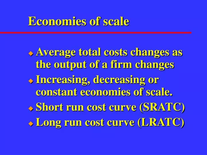
Economies of scale • Average total costs changes as the output of a firm changes • Increasing, decreasing or constant economies of scale. • Short run cost curve (SRATC) • Long run cost curve (LRATC)
Constant economies of scale Cost SRATC1 SRATC2 LRATC Q2 Q Q1
Increasing economies of scale Cost SRATC1 SRATC2 LRATC Q1 Q2 Q
Decreasing economies of scale Cost SRATC2 SRATC1 LRATC Q1 Q2 Q
US Pork Sector Study Financial results for 2000 Net Profit Breakeven Net Loss 1-2 65% 24% 11% 2-3 77% 15% 8% 3-5 79% 16% 5% 5-10 78% 13% 9% 10-50 77% 12% 11% 50-500 90% 5% 5% 500+ 95% 5% 0%
US Pork Sector StudyStay in price until 2003 (%) 1000 hd $36 $39 $42 $45 $48 1-2 16 36 69 86 90 2-3 18 42 71 87 97 3-5 18 39 70 90 94 5-10 16 39 75 92 98 10-50 22 49 74 91 96 50-500 4 61 88 97 99 500+ 28 50 89 94 100
Processing cost curves Specialized plants High fixed cost Cost SRATC Q
So what??? • Short run price implications • Supply chain management • Open market or contract • Packing plants • Ethanol plants • Soybean processing • Biodiesel
Externalities and cost curves Cost Cost curve exhibiting increasing economies of scale Q
Externalities and cost curves Cost Cost curve with external cost internalized to the firm Q
Supply and Demand summary • Demand originates with individual consumer’s utility and budget constraint • Supply originates with individual firm’s marginal cost curve
Consumption is not demand • Consumption = • Beginning stocks + production + imports • – exports – ending stocks • Government reports of inventory • Per capita consumption = • consumption / population
Equilibrium P and Q Equilibrium price is where Qs = Qd. P S Pe D Qe Q
Price elasticity • A measure of responsiveness of the quantity supplied or demanded to changes in prices. • Percentage change in quantity for a 1% change in price.
Elasticity of demand Q / Q P / P Ep = Q P Ep = x Q P Q0 - Q1 P0 + P1 Ep = x Q0 + Q1 P0 - P1
Price elasticity and curves • Ep changes along a sloping demand or supply curve • Special exceptions
Relative measures • |Ep| > 1 elastic • |Ep| = 1 unitary elastic • |Ep| < 1 inelastic
Price elasticity & total revenue • TR = P x Q • Elastic demand • P and TR inversely related • Inelastic demand • P and TR directly related
Price elasticity & total revenue P Elastic Inelastic Q
So what???? Where are you on the demand curve? P 60 55 20 15 Q 7 10 11 6
Income elasticity • Percentage change in quantity for a 1% change in income • Positive for most food items • Relatively small i.e., 0.2 Q I Ei = x Q I
Cross-price elasticity • Percentage change in quantity for a 1% change in price of a substitute or complement • Positive or negative • Much smaller than Ep Qk Pj Epj = x Qk Pj
Examples of Ag elasticities Ep Ei Beef -.62 .45 Pork -.73 .44 Chicken -.53 .36 Milk -.26 -.22 Grapes -1.38 .44 Lettuce -.14 .23
Own and Cross Price Elasticities Ep of demand for beef Beef -.62 Pork .11 Lamb .01 Chicken .06 Other -.01 Income .45
Net change in quantity • Net effect of changes in own price, cross price, and income multiplied by the appropriate elasticities. • Addresses the fact that not all else is equal.
Elasticities at various markets • The greater the number of substitutes the more elastic the demand. • For a given Q, look at % P • More elastic at retail level
Elasticities at market levels P Hy-Vee T-bone in Ames Hy-Vee T-bone All T-bone All meat All beef All food Q
Derived Demand • The demand for inputs that are used to produce the final products. • Examples: • Flour => wheat • Soybean meal => soybeans • Fed cattle => feeder cattle
Derived Demand P Retail pork chop demand Wholesale pork demand Farm level demand for hogs Demand for corn to feed hogs Demand for inputs to produce corn Q
Elasticities at retail and farm Dd = f (Dd, M) S P PR M PF DRetail = Primary DFarm = Derived Q Qe
Elasticity Summary • Relationship between Q and P • Changes along demand curve • Elasticity and total revenue • Cross-price and income elasticities • Relative size • Own, cross, and income • Farm v. retail