Download
1 / 42
420 likes | 537 Views
Randomized Online Algorithm for Minimum Metric Bipartite Matching. Adam Meyerson UCLA. A Recent Result. Randomized Online Algorithm for Minimum Metric Bipartite Matching. Joint work with two UCLA students (one recently graduated): Akash Nanavati and Laura Poplawski.

E N D
Randomized Online Algorithm for Minimum Metric Bipartite Matching Adam Meyerson UCLA
A Recent Result • Randomized Online Algorithm for Minimum Metric Bipartite Matching. • Joint work with two UCLA students (one recently graduated): Akash Nanavati and Laura Poplawski. • Recently presented at Symposium on Discrete Algorithms (SODA) 2006.
Bipartite Matching • Pair up each red node with a blue node. • One-to-one pairing. • Each pair of nodes must have an edge between them.
Bipartite Matching • Pair up each red node with a blue node. • One-to-one pairing. • Each pair of nodes must have an edge between them.
Min-Cost Bipartite Matching • Each edge has a cost. • Find a matching of red nodes with blue nodes. • Minimize the total cost of the edges between matched pairs.
Importance of Matching • Task assignment problems. • Measuring data similarity. • Relationship to network flow. • Subroutine in many other algorithms.
Online Matching • We’re given only the red nodes. • Blue nodes are designated one at a time. • As each blue nodes is designated we must match it to an unmatched red node.
Why Online Matching? • Assigning tasks to consultants (or jobs to machines without migration). • Updating existing matchings “on the fly” without making major modifications. • Possible subroutine for other online problems.
Simplifying the Problem • We can assume that distances between nodes form a metric. • Satisfy symmetry: d(x,y)=d(y,x) • Satisfy triangle inequality: d(x,y)+d(y,z) ≥ d(x,z) • This assumption will hold for distances on a surface (for example) and is common for many problems (like traveling salesman).
Measuring Success • After all the nodes have arrived, we will have some final matching M. Let the cost of this matching be C(M). • If we had known all the red and blue nodes initially, we could compute the minimum-cost matching M*. • The competitive ratio of our algorithm is the maximum, over all sequences of blue nodes, of C(M)/C(M*). We would like this to be small.
Some Points about the Model • We will allow co-located red and blue nodes. These can be matched for cost zero (they are distance zero apart). • Not every node needs to be either red or blue; there could be nodes of the graph which are not supposed to be matched. • The underlying metric could be infinite (for example the Euclidean plane) provided distances can be computed easily.
“Obvious” Solution: Greedy • When a blue node is designated, match it to the closest unmatched red node. • Simple, easy to implement. • How could we do better? • Yet, there is a sequence of inputs (a graph, set of red nodes, and ordered set of blue nodes) such that greedy gives a very bad solution.
Greed is Bad 2 2 4 8 ….
Greed is Bad 2 2 4 8 ….
Greed is Bad 2 2 4 8 ….
Greed is Bad 2 2 4 8 ….
How bad is greedy? • We pay 1+2+4+8… = 2k in total. • k = number of red nodes • The best (minimum-cost) matching would pay only a cost of 1. • So greedy is really bad in the worst case!
Is there a better algorithm? • Permutation algorithm • Khuller, Mitchell, Vazirani ToCS 1994. • At worst (2k-1) times the best matching. • But isn’t a (2k-1) factor really bad? • It seems that no algorithm can do better…
Eventual Cost Comparison • Our Algorithm pays 2k-1. • Optimum pays only 1. • How did this happen? • “Adversary” always knew which red node we would match up. • Next blue node designated is always really close to the last red node we matched.
Onward to New Results! • This matching 2k-1 competitive result is all that was previously known. • People started to work on special kinds of graphs… • We consider randomized algorithms. • “Adversary” does not know our coin flips in advance! • Randomization has helped in the past for other online problems (paging).
Our Result • Joint work with Akash Nanavati and Laura Poplawski. • We design a randomized online algorithm which obtains O(log3 k) competitive matching. • Dramatically better for large k.
Greedy Returns! • Our algorithm is a randomized greedy. • As each blue node is designated, match to the closest unmatched red node. • If there’s a tie, break it by choosing uniformly at random.
But greedy doesn’t work… • The same bad example from before will kill us (again). • But greedy does work on some special graphs. • On the star example, randomized greedy will cost an expected O(log k) times the optimum.
Our Main Theorem • Randomized greedy works on a -HST. • This is a tree where: • All children of a node equidistant from that node. • Distance from child to parent is (1/) times distance from parent to grandparent. 2 1
The Inductive Step • Consider the root of the tree. • Let mi be the difference between number of red, blue nodes in subtree i. • OPT must match at least M=∑mi/2 outside. • We will bound the number we match outside subtree online.
The Key Lemma • Let mi* be the number of blue nodes from subtree i which our algorithm matches outside subtree i. • We will show that ∑mi*≤ 2M ln k + 1 • Here k = total number of blue nodes. • Pf: Let t=number of blue nodes matched outside when t blue nodes yet to arrive. • Let t=∑ 2 ln x. This sum is over i such that a future blue node will arrive which cannot be matched to a red node within its subtree.
Completing Lemma Proof • Initially, t+t ≤ 2M ln k. • At each time step, the value of t can only change if we match a node outside its subtree. At this point we might “bump” a later node by matching to its designated red node (i.e. we pick the wrong subtree). The new value for the potential is: E[t-1] ≤ t-1. • We conclude that at termination, we have the required bound.
Using the Lemma • We can bound the total cost of the matching by the cost of nodes matched outside their subtree, plus the cost of matching within the subtrees. This second value can be bounded using induction. • The cost of matching within the subtrees cannot be directly compared to optimum, because outside nodes matched within the subtree might be matched to the “wrong” places.
Completing the Proof • CostOPT(T) = ∑iCostOPT(Si) + 2M • CostUS(T) ≤ ∑iCostUS(Si*) + ∑imi*(2) • Here Si* represents the set of red and blue nodes in Si not matched outside the tree. • is the ratio of the sum of all distances from leaf to root between one level and the next (this can be bounded easily in terms of ).
Applying Induction • If we have a competitive ratio of R, we can conclude that CostUS(Si*)≤R CostOPT(Si*) inductively. It remains to relate the cost of Si* to that of Si. • We could try to match to the same places as OPT does; the problem is “wrong” matches from outside. However, there are at most mi* such wrong matches. Each costs no more than 2 to correct. • CostUS(Si*) ≤ R(CostOPT(Si) + 2mi*)
Finishing HST Result • Now it’s just a matter of algebra and solving for R. • We manage to show that: • O(log k)-competitive on -HST • Require that ≥(log k) • These bounds on performance of randomized greedy on k-HST are tight; to improve the result a new algorithm would be needed.
So what? • -HST is not a very general graph. • However, there is series of recent results on metric embeddings. • In particular, result of Fakcharoenphol, Rao, and Talwar in STOC 2003. • Any metric can be transformed via a randomized mapping into an -HST, such that no distance is contracted, and the expected expansion of any distance is at most O( log n).
Randomized Online Matching! • Transform the original metric using the [FRT] result into a (log k)-HST. • Use randomized greedy to match blue nodes with red nodes as they arrive, based on the (random) distances in the HST. • Expected cost of matching will be within O(log2 k log n) of optimum
A Simple Trick • We actually only care about maintaining the relative positions of red nodes. This enables us to use a simple trick (matching blue nodes via the nearest red node neighbor) to improve the result to O(log3 k).
Future Work (in progress) • We hope to design a good randomized algorithm for k-server. • Police cars at various locations, emergencies arise one at a time, must move a police car to each emergency. • Similar to matching, but can move the same police car multiple times. • Again 2k-1 result known (deterministic) but randomized may be able to do better!